High-dimensional Bayesian optimization with Random EMbedding Bayesian Optimization (REMBO).#
This notebook demonstrates a simple method for optimizing a high-dimensional (100-D) problem, where standard BO methods have trouble.
[1]:
import math
import gpflow
import numpy as np
import tensorflow as tf
import tensorflow_probability as tfp

np.random.seed(1793)
tf.random.set_seed(1793)
Describe the problem#
In this example, we augment the standard two-dimensional Michalewicz function with 98 dummy dimensions to obtain a 100-dimensional problem over the hypercube \([0, \pi]^{100}\).
We compare three approaches to optimizing this problem. The first uses a standard GP model over all 100 dimensions, using expected improvement as our acquisition function. As standard Gaussian process models have trouble modeling high dimensional data, we do not expect this approach to perform well. Therefore, we compare this to two Random EMbedding Bayesian Optimization (REMBO; see [WZH+13]) approaches.
Instead of training a GP model and optimizing an acquisition function on the high-dimensional space directly, REMBO constructs a low-dimensional search space, performing the modeling and acquisition on this space. In order to transfer to the high-dimensional space, REMBO uses a static random projection matrix \(A \in \mathbb{R}^{D \times d}\) to project query points from the lower, \(d\)-dimensional space to the original higher, \(D\)-dimensional space.
As the lower dimension \(d\) is a choice, we compare \(d = 2\) and \(d = 5\). While \(d = 2\) should be sufficient (as the problem is intrinsically two-dimensional), a higher dimension may improve the chance of a good random embedding being found, at the cost of making it more difficult to find good areas of the lower-dimensional search space.
We run each method 5 times to ensure that the results are not due to luck.
[2]:
from trieste.objectives.single_objectives import Michalewicz2
from trieste.space import Box
from trieste.models.gpflow import GaussianProcessRegression

# Set the dimension of the full problem
D = 100

num_initial_points = 2
num_steps = 48
num_seeds = 5

objective = Michalewicz2.objective
minimum = Michalewicz2.minimum
search_space = (
    Box([0.0], [math.pi]) ** D
)  # manually construct the high-dimensional search space


# We simply add dummy dimensions to create the new objective
def high_dim_objective(x):
    tf.debugging.assert_shapes([(x, (..., D))])

    return objective(x[..., :2])


def build_model(data, d):
    # add a bit of noise, since there's a risk the variance could be zero for Michalewicz
    variance = tf.math.reduce_variance(data.observations) + 1e-4
    kernel = gpflow.kernels.Matern52(variance=variance, lengthscales=[0.2] * d)
    prior_scale = tf.cast(1.0, dtype=tf.float64)
    kernel.variance.prior = tfp.distributions.LogNormal(
        tf.cast(-2.0, dtype=tf.float64), prior_scale
    )
    kernel.lengthscales.prior = tfp.distributions.LogNormal(
        tf.math.log(kernel.lengthscales), prior_scale
    )
    gpr = gpflow.models.GPR(data.astuple(), kernel, noise_variance=1e-5)
    gpflow.set_trainable(gpr.likelihood, False)

    return GaussianProcessRegression(gpr, num_kernel_samples=100)
Run standard Bayesian optimization#
We run the process 5 times - note that this takes a while!
[3]:
import trieste

final_datasets = []  # to store the results

observer = trieste.objectives.utils.mk_observer(high_dim_objective)

for _ in range(num_seeds):
    # Sample initial points
    initial_query_points = search_space.sample_sobol(num_initial_points)
    initial_data = observer(initial_query_points)

    # Build the model over the high-dimensional space
    model = build_model(initial_data, d=D)

    # Set up the optimizer and run the loop
    bo = trieste.bayesian_optimizer.BayesianOptimizer(observer, search_space)

    # Store the results
    result = bo.optimize(num_steps, initial_data, model)
    dataset = result.try_get_final_dataset()

    final_datasets.append(dataset)
Optimization completed without errors
Optimization completed without errors
Optimization completed without errors
Optimization completed without errors
Optimization completed without errors
We now show how to implement REMBO, by providing a new observer that acts on a projection of the input data by wrapping the original objective.
[4]:
def make_REMBO_observer_and_search_space(
    full_dim, low_dim, objective, search_space
):
    assert isinstance(search_space, Box)

    A = tf.random.normal(
        [full_dim, low_dim], dtype=gpflow.default_float()
    )  # sample projection matrix

    new_search_space = Box(
        [-math.sqrt(low_dim)] * low_dim, [math.sqrt(low_dim)] * low_dim
    )  # recommendation from REMBO paper

    def new_objective(y):
        tf.debugging.assert_shapes([(y, (..., low_dim))])

        rescaled_search_space = Box(
            [-1.0] * full_dim, [1.0] * full_dim
        )  # REMBO assumes the original space has bounds [-1, 1]^full_dim

        scaling = (search_space.upper - search_space.lower) / (
            rescaled_search_space.upper - rescaled_search_space.lower
        )

        x = tf.clip_by_value(
            tf.matmul(y, A, transpose_b=True),
            clip_value_min=-1,
            clip_value_max=1,
        )  # project into the new box

        x_rescaled = (
            x - rescaled_search_space.lower
        ) * scaling + search_space.lower  # rescale to match the original search space

        return objective(x_rescaled)

    observer = trieste.objectives.utils.mk_observer(new_objective)

    return observer, new_search_space
Using the new observer, the process remains the same as before, except that now we must choose \(d\) and build a model for that dimension. We run the same experiment for \(d=2\) and \(d=5\).
[5]:
d = 2
rembo_2_final_datasets = []

for _ in range(num_seeds):
    rembo_observer, rembo_search_space = make_REMBO_observer_and_search_space(
        D, d, high_dim_objective, search_space
    )

    initial_query_points = rembo_search_space.sample_sobol(num_initial_points)
    initial_data = rembo_observer(initial_query_points)

    model = build_model(initial_data, d=d)

    bo = trieste.bayesian_optimizer.BayesianOptimizer(
        rembo_observer, rembo_search_space
    )

    result = bo.optimize(num_steps, initial_data, model)
    dataset = result.try_get_final_dataset()

    rembo_2_final_datasets.append(dataset)
Optimization completed without errors
Optimization completed without errors
Optimization completed without errors
Optimization completed without errors
Optimization completed without errors
We repeat the above but with d=5 - this might help find more suitable projections.
[6]:
d = 5
rembo_5_final_datasets = []

for _ in range(num_seeds):
    rembo_observer, rembo_search_space = make_REMBO_observer_and_search_space(
        D, d, high_dim_objective, search_space
    )

    initial_query_points = rembo_search_space.sample_sobol(num_initial_points)
    initial_data = rembo_observer(initial_query_points)

    model = build_model(initial_data, d=d)

    bo = trieste.bayesian_optimizer.BayesianOptimizer(
        rembo_observer, rembo_search_space
    )

    result = bo.optimize(num_steps, initial_data, model)
    dataset = result.try_get_final_dataset()

    rembo_5_final_datasets.append(dataset)
Optimization completed without errors
Optimization completed without errors
Optimization completed without errors
Optimization completed without errors
Optimization completed without errors
We produce a regret plot below for each method.
[7]:
import matplotlib.pyplot as plt

_, ax = plt.subplots(1, 3)

for i in range(num_seeds):
    observations = final_datasets[i].observations.numpy()
    suboptimality = observations - minimum.numpy()
    ax[0].plot(np.minimum.accumulate(suboptimality))
    ax[0].axvline(x=num_initial_points - 0.5, color="tab:blue")
    ax[0].set_yscale("log")
    ax[0].set_ylabel("Regret")
    ax[0].set_ylim(0.001, 100)
    ax[0].set_xlabel("# evaluations")
    ax[0].set_title("Full-D BO")

    rembo_observations = rembo_2_final_datasets[i].observations.numpy()
    suboptimality = rembo_observations - minimum.numpy()
    ax[1].plot(np.minimum.accumulate(suboptimality))
    ax[1].axvline(x=num_initial_points - 0.5, color="tab:blue")
    ax[1].set_yscale("log")
    ax[1].set_ylim(0.001, 100)
    ax[1].set_yticks([])
    ax[1].set_xlabel("# evaluations")
    ax[1].set_title("REMBO: d=2")

    rembo_5_observations = rembo_5_final_datasets[i].observations.numpy()
    suboptimality = rembo_5_observations - minimum.numpy()
    ax[2].plot(np.minimum.accumulate(suboptimality))
    ax[2].axvline(x=num_initial_points - 0.5, color="tab:blue")
    ax[2].set_yscale("log")
    ax[2].set_ylim(0.001, 100)
    ax[2].set_yticks([])
    ax[2].set_xlabel("# evaluations")
    ax[2].set_title("REMBO: d=5")
/opt/hostedtoolcache/Python/3.10.12/x64/lib/python3.10/site-packages/matplotlib/_mathtext.py:1880: UserWarning: warn_name_set_on_empty_Forward: setting results name 'sym' on Forward expression that has no contained expression
  - p.placeable("sym"))
/opt/hostedtoolcache/Python/3.10.12/x64/lib/python3.10/site-packages/matplotlib/_mathtext.py:1885: UserWarning: warn_ungrouped_named_tokens_in_collection: setting results name 'name' on ZeroOrMore expression collides with 'name' on contained expression
  "{" + ZeroOrMore(p.simple | p.unknown_symbol)("name") + "}")
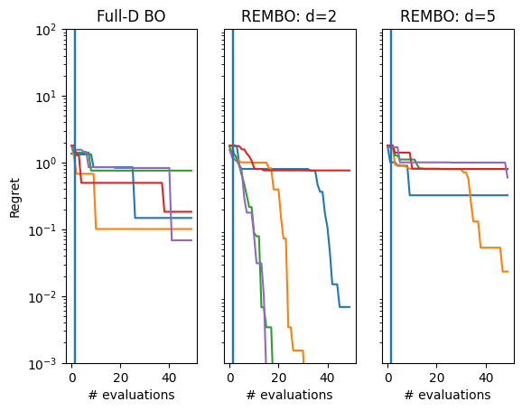
We see that REMBO with \(d=2\) generally performs the best, whereas both the full-dimensional approach and \(d=5\) struggle more.