[1]:
import gpflow.kernels
Multifidelity Modelling with Autoregressive Model#
This tutorial demonstrates the usage of the MultifidelityAutoregressive model for fitting multifidelity data. This is an implementation of the AR1 model initially described in [KOHagan00].
[2]:
import tensorflow as tf
import numpy as np
import matplotlib.pyplot as plt

np.random.seed(1793)
tf.random.set_seed(1793)
Describe the problem#
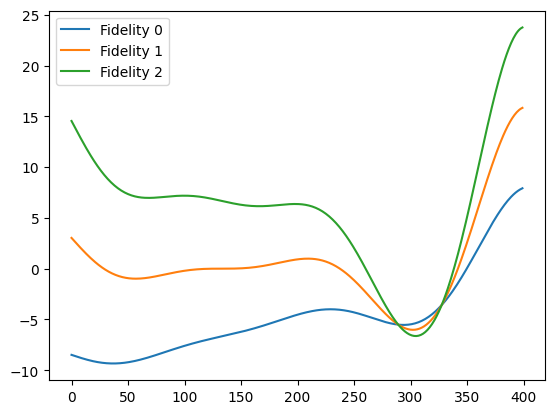
In this tutorial we will consider the scenario where we have a simulator that can be run at three fidelities, with the ability to get cheap but coarse results at the lowest fidelity, more expensive but more refined results at a middle fidelity and very accurate but very expensive results at the highest fidelity.
We define the true functions for the fidelities as:
Note that noise is optionally added to any observations in all but the lowest fidelity. There are a few modelling assumptions: 1. The lowest fidelity is noise-free 2. The data is cascading, e.g any point that has an observation at a high fidelity also has one at the lower fidelities.
[3]:
# Define the multifidelity simulator
def linear_simulator(x_input, fidelity, add_noise=False):
    f = 0.5 * ((6.0 * x_input - 2.0) ** 2) * tf.math.sin(
        12.0 * x_input - 4.0
    ) + 10.0 * (x_input - 1.0)
    f = f + fidelity * (f - 20.0 * (x_input - 1.0))
    if add_noise:
        noise = tf.random.normal(f.shape, stddev=1e-1, dtype=f.dtype)
    else:
        noise = 0
    f = tf.where(fidelity > 0, f + noise, f)
    return f


# Plot the fidelities
x = np.linspace(0, 1, 400)

y0 = linear_simulator(x, 0)
y1 = linear_simulator(x, 1)
y2 = linear_simulator(x, 2)

plt.plot(y0, label="Fidelity 0")
plt.plot(y1, label="Fidelity 1")
plt.plot(y2, label="Fidelity 2")
plt.legend()
plt.show()
Trieste handles fidelities by adding an extra column to the data containing the fidelity information of the query point. The function check_and_extract_fidelity_query_points will check that the fidelity column is valid, and if so, will separate the query points and the fidelity information.
[4]:
from trieste.data import Dataset, check_and_extract_fidelity_query_points


# Create an observer class to deal with multifidelity input query points
class Observer:
    def __init__(self, simulator):
        self.simulator = simulator

    def __call__(self, x, add_noise=True):
        # Extract raw input and fidelity columns
        x_input, x_fidelity = check_and_extract_fidelity_query_points(x)

        # note: this assumes that my_simulator broadcasts, i.e. accept matrix inputs.
        # If not you need to replace this by a for loop over all rows of "input"
        observations = self.simulator(x_input, x_fidelity, add_noise)
        return Dataset(query_points=x, observations=observations)


# Instantiate the observer
observer = Observer(linear_simulator)
Now we can define the other parameters of our problem, such as the input dimension, search space and number of fidelities.
[5]:
from trieste.space import Box

input_dim = 1
n_fidelities = 3

lb = np.zeros(input_dim)
ub = np.ones(input_dim)

input_search_space = Box(lb, ub)
Create initial dataset#
[6]:
from trieste.data import add_fidelity_column
# Define sample sizes of low, mid and high fidelities
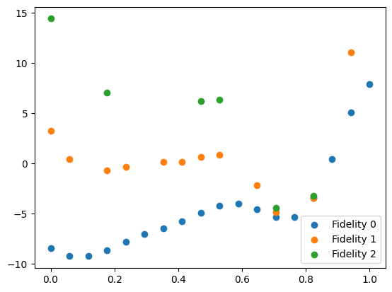
sample_sizes = [18, 12, 6]
xs = [tf.linspace(0, 1, sample_sizes[0])[:, None]]
# Take a subsample of each lower fidelity to sample at the next fidelity up
for fidelity in range(1, n_fidelities):
samples = tf.Variable(
np.random.choice(
xs[fidelity - 1][:, 0], size=sample_sizes[fidelity], replace=False
)
)[:, None]
xs.append(samples)
# Add fidelity columns to training data
initial_samples_list = [add_fidelity_column(x, i) for i, x in enumerate(xs)]
initial_sample = tf.concat(initial_samples_list, 0)
initial_data = observer(initial_sample, add_noise=True)
We can plot the initial data. We separate the dataset into individual fidelities using the split_dataset_by_fidelity function.
[7]:
from trieste.data import split_dataset_by_fidelity

data = split_dataset_by_fidelity(initial_data, num_fidelities=n_fidelities)

plt.scatter(data[0].query_points, data[0].observations, label="Fidelity 0")
plt.scatter(data[1].query_points, data[1].observations, label="Fidelity 1")
plt.scatter(data[2].query_points, data[2].observations, label="Fidelity 2")
plt.legend()
plt.show()
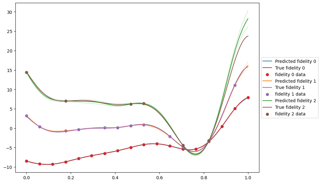
Fit AR(1) model#
Now we can fit the MultifidelityAutoregressive model to this data. We use the build_multifidelity_autoregressive_models to create the sub-models required by the multifidelity model.
[8]:
from trieste.models.gpflow import (
    MultifidelityAutoregressive,
    build_multifidelity_autoregressive_models,
)

# Initialise model
multifidelity_model = MultifidelityAutoregressive(
    build_multifidelity_autoregressive_models(
        initial_data, n_fidelities, input_search_space
    )
)

# Update and optimize model
multifidelity_model.update(initial_data)
multifidelity_model.optimize(initial_data)
Plot Results#
Now we can plot the results to have a look at the fit. The MultifidelityAutoregressive.predict method requires data with a fidelity column that specifies the fidelity for each data point to be predicted at. We use the add_fidelity_column function to add this.
[9]:
X = tf.linspace(0, 1, 200)[:, None]
X_list = [add_fidelity_column(X, i) for i in range(n_fidelities)]
predictions = [multifidelity_model.predict(x) for x in X_list]

fig, ax = plt.subplots(1, 1, figsize=(10, 7))

pred_colors = ["tab:blue", "tab:orange", "tab:green"]
gt_colors = ["tab:red", "tab:purple", "tab:brown"]

for fidelity, prediction in enumerate(predictions):
    mean, var = prediction
    ax.plot(
        X,
        mean,
        label=f"Predicted fidelity {fidelity}",
        color=pred_colors[fidelity],
    )
    ax.plot(
        X,
        mean + 1.96 * tf.math.sqrt(var),
        alpha=0.2,
        color=pred_colors[fidelity],
    )
    ax.plot(
        X,
        mean - 1.96 * tf.math.sqrt(var),
        alpha=0.2,
        color=pred_colors[fidelity],
    )
    ax.plot(
        X,
        observer(X_list[fidelity], add_noise=False).observations,
        label=f"True fidelity {fidelity}",
        color=gt_colors[fidelity],
    )
    ax.scatter(
        data[fidelity].query_points,
        data[fidelity].observations,
        label=f"fidelity {fidelity} data",
        color=gt_colors[fidelity],
    )
ax.legend(loc="center left", bbox_to_anchor=(1, 0.5))
plt.show()
Comparison with naive model fit on high fidelity#
We can compare with a model that was fit just on the high fidelity data, and see the gains from using the low fidelity data.
[10]:
from trieste.models.gpflow import GaussianProcessRegression, build_gpr
from trieste.data import add_fidelity_column

# Get high fidleity data
hf_data = data[2]

# Fit simple gpr model to high fidelity data
gpr_model = GaussianProcessRegression(build_gpr(hf_data, input_search_space))

gpr_model.update(hf_data)
gpr_model.optimize(hf_data)

X = tf.linspace(0, 1, 200)[:, None]
# Turn X into high fidelity query points for the multifidelity model
X_for_multifid = add_fidelity_column(X, 2)

gpr_predictions = gpr_model.predict(X)
multifidelity_predictions = multifidelity_model.predict(X_for_multifid)

fig, ax = plt.subplots(1, 1, figsize=(10, 7))

"tab:blue", "tab:orange", "tab:green"

# Plot gpr results
mean, var = gpr_predictions
ax.plot(X, mean, label=f"GPR", color="tab:blue")
ax.plot(X, mean + 1.96 * tf.math.sqrt(var), alpha=0.2, color="tab:blue")
ax.plot(X, mean - 1.96 * tf.math.sqrt(var), alpha=0.2, color="tab:blue")

# Plot gpr results
mean, var = multifidelity_predictions
ax.plot(X, mean, label=f"MultifidelityAutoregressive", color="tab:orange")
ax.plot(X, mean + 1.96 * tf.math.sqrt(var), alpha=0.2, color="tab:orange")
ax.plot(X, mean - 1.96 * tf.math.sqrt(var), alpha=0.2, color="tab:orange")


# Plot true function
ax.plot(
    X,
    observer(X_for_multifid, add_noise=False).observations,
    label=f"True function",
    color="tab:green",
)

# Scatter the data
ax.scatter(
    hf_data.query_points, hf_data.observations, label=f"Data", color="tab:green"
)
plt.legend()
plt.show()
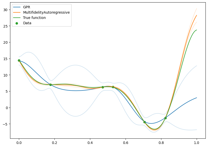
It’s clear that there is a large benefit to being able to make use of the low fidelity data, and this is particularly noticable in the greatly reduced confidence intervals.
A more complex model for non-linear problems#
A more complex multifidelity model (NARGP, here MultifidelityNonlinearAutoregressive), originally proposed in :cite:perdikaris2017nonlinear is also available, to tackle the case where the relation between fidelities is strongly non-linear.
We start by defining a new multi-fidelity problem, with two fidelities, for \(x \in [0,1]\):
Contrary to the previous case, the high-fidelity level follows the square of the low-fidelity one. As the low fidelity values oscillate between positive and negative ones, it makes inferring this relationship particularly difficult for the AR(1) model, as we see below.
As previously, we create an observer, and some initial data.
[11]:
def nonlinear_simulator(x_input, fidelity, add_noise):
    bad_fidelities = tf.math.logical_and(fidelity != 0, fidelity != 1)
    if tf.math.count_nonzero(bad_fidelities) > 0:
        raise ValueError(
            "Nonlinear simulator only supports 2 fidelities (0 and 1)"
        )
    else:
        f = tf.math.sin(8 * np.pi * x_input)
        fh = (
            x_input - tf.sqrt(tf.Variable(2.0, dtype=tf.float64))
        ) * tf.square(f)
        f = tf.where(fidelity > 0, fh, f)

        if add_noise:
            f += tf.random.normal(f.shape, stddev=1e-2, dtype=f.dtype)

        return f


observation_noise = True
observer = Observer(nonlinear_simulator)

n_fidelities = 2
sample_sizes = [50, 14]

xs = [tf.linspace(0, 1, sample_sizes[0])[:, None]]
xh = tf.Variable(
    np.random.choice(xs[0][:, 0], size=sample_sizes[1], replace=False)
)[:, None]
xs.append(xh)

initial_samples_list = [
    tf.concat([x, tf.ones_like(x) * i], 1) for i, x in enumerate(xs)
]
initial_sample = tf.concat(initial_samples_list, 0)
initial_data = observer(initial_sample, add_noise=observation_noise)
We create an AR(1) model as before, and use the build_multifidelity_nonlinear_autoregressive_models to create the NARGP. We then train both model on the same data.
[12]:
from trieste.models.gpflow import (
    MultifidelityNonlinearAutoregressive,
    build_multifidelity_nonlinear_autoregressive_models,
)

ar1 = MultifidelityAutoregressive(
    build_multifidelity_autoregressive_models(
        initial_data, n_fidelities, input_search_space
    )
)
nargp = MultifidelityNonlinearAutoregressive(
    build_multifidelity_nonlinear_autoregressive_models(
        initial_data, n_fidelities, input_search_space
    )
)

ar1.update(initial_data)
ar1.optimize(initial_data)

nargp.update(initial_data)
nargp.optimize(initial_data)
Now we can plot the two model predictions.
[13]:
data = split_dataset_by_fidelity(initial_data, n_fidelities)

X = tf.linspace(0, 1, 200)[:, None]
X_list = [tf.concat([X, tf.ones_like(X) * i], 1) for i in range(n_fidelities)]
predictions_ar1 = [ar1.predict(x) for x in X_list]
predictions_nargp = [nargp.predict(x) for x in X_list]
fig, ax = plt.subplots(2, 1, figsize=(10, 7))
for ax_id, model_predictions in enumerate([predictions_ar1, predictions_nargp]):
    for fidelity, prediction in enumerate(model_predictions):
        mean, var = prediction
        ax[ax_id].plot(X, mean, label=f"Predicted fidelity {fidelity}")
        ax[ax_id].plot(X, mean + 1.96 * tf.math.sqrt(var), alpha=0.2)
        ax[ax_id].plot(X, mean - 1.96 * tf.math.sqrt(var), alpha=0.2)
        ax[ax_id].plot(
            X,
            observer(X_list[fidelity], add_noise=False).observations,
            label=f"True fidelity {fidelity}",
        )
        ax[ax_id].scatter(
            data[fidelity].query_points,
            data[fidelity].observations,
            label=f"fidelity {fidelity} data",
        )
        ax[ax_id].title.set_text(
            "MultifidelityAutoregressive" if ax_id == 0 else "NARGP"
        )
    ax[ax_id].legend(loc="center left", bbox_to_anchor=(1, 0.5))
fig.suptitle("Non-Linear Problem")
plt.show()
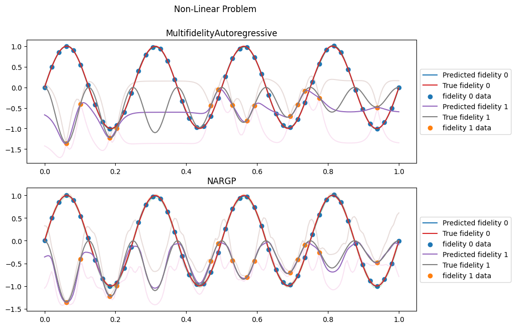
The AR(1) model is incapable of using the lower fidelity data and its prediction for the high fidelity level simply returns to the prior when there is no high-fidelity data. In contrast, the NARGP model clearly captures the non-linear relashionship and is able to predict accurately the high-fideility level everywhere.