Explicit Constraints#
This notebook demonstrates ways to perfom Bayesian optimization with Trieste in the presence of explicit input constraints.
[1]:
import matplotlib.pyplot as plt
import numpy as np
import tensorflow as tf

import trieste

np.random.seed(1234)
tf.random.set_seed(1234)
Describe the problem#
In this example, we consider the same problem presented in our EI notebook, i.e. seeking the minimizer of the two-dimensional Branin function, but with input constraints.
There are 3 linear constraints with respective lower/upper limits (i.e. 6 linear inequality constraints). There are 2 non-linear constraints with respective lower/upper limits (i.e. 4 non-linear inequality constraints).
We begin our optimization after collecting five function evaluations from random locations in the search space.
[2]:
from trieste.acquisition.function import fast_constraints_feasibility
from trieste.objectives import ScaledBranin
from trieste.objectives.utils import mk_observer
from trieste.space import Box, LinearConstraint, NonlinearConstraint

observer = mk_observer(ScaledBranin.objective)


def _nlc_func0(x):
    c0 = x[..., 0] - 0.2 - tf.sin(x[..., 1])
    c0 = tf.expand_dims(c0, axis=-1)
    return c0


def _nlc_func1(x):
    c1 = x[..., 0] - tf.cos(x[..., 1])
    c1 = tf.expand_dims(c1, axis=-1)
    return c1


constraints = [
    LinearConstraint(
        A=tf.constant([[-1.0, 1.0], [1.0, 0.0], [0.0, 1.0]]),
        lb=tf.constant([-0.4, 0.15, 0.2]),
        ub=tf.constant([0.5, 0.9, 0.9]),
    ),
    NonlinearConstraint(_nlc_func0, tf.constant(-1.0), tf.constant(0.0)),
    NonlinearConstraint(_nlc_func1, tf.constant(-0.8), tf.constant(0.0)),
]

unconstrained_search_space = Box([0, 0], [1, 1])
constrained_search_space = Box([0, 0], [1, 1], constraints=constraints)  # type: ignore

num_initial_points = 5
initial_query_points = constrained_search_space.sample(num_initial_points)
initial_data = observer(initial_query_points)
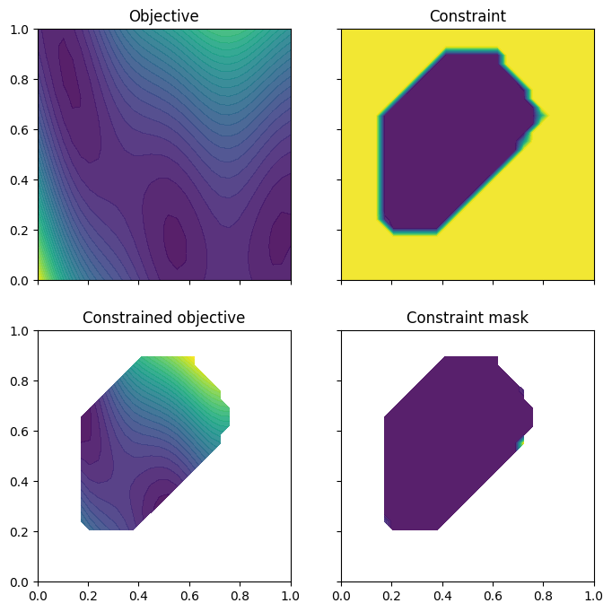
We wrap the objective and constraint functions as methods on the Sim class. This provides us one way to visualise the objective function, as well as the constrained objective. We get the constrained objective by masking out regions where the constraint function is above the threshold.
[3]:
from trieste.experimental.plotting import plot_objective_and_constraints


class Sim:
    threshold = 0.5

    @staticmethod
    def objective(input_data):
        return ScaledBranin.objective(input_data)

    @staticmethod
    def constraint(input_data):
        # `fast_constraints_feasibility` returns the feasibility, so we invert it. The plotting
        # function masks out values above the threshold.
        return 1.0 - fast_constraints_feasibility(constrained_search_space)(
            input_data
        )


plot_objective_and_constraints(constrained_search_space, Sim)
plt.show()
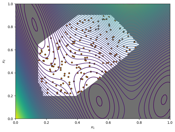
In addition to the normal sampling methods, the search space provides sampling methods that return feasible points only. Here we demonstrate sampling 200 feasible points from the Halton sequence. We can visualise the sampled points along with the objective function and the constraints.
[4]:
from trieste.experimental.plotting import plot_function_2d

[xi, xj] = np.meshgrid(
    np.linspace(
        constrained_search_space.lower[0],
        constrained_search_space.upper[0],
        100,
    ),
    np.linspace(
        constrained_search_space.lower[1],
        constrained_search_space.upper[1],
        100,
    ),
)
xplot = np.vstack(
    (xi.ravel(), xj.ravel())
).T  # Change our input grid to list of coordinates.
constraint_values = np.reshape(
    constrained_search_space.is_feasible(xplot), xi.shape
)

_, ax = plot_function_2d(
    ScaledBranin.objective,
    constrained_search_space.lower,
    constrained_search_space.upper,
    contour=True,
)

points = constrained_search_space.sample_halton_feasible(200)

ax[0, 0].scatter(
    points[:, 0],
    points[:, 1],
    s=15,
    c="tab:orange",
    edgecolors="black",
    marker="o",
)

ax[0, 0].contourf(
    xi,
    xj,
    constraint_values,
    levels=1,
    colors=[(0.2, 0.2, 0.2, 0.7), (1, 1, 1, 0)],
    zorder=1,
)

ax[0, 0].set_xlabel(r"$x_1$")
ax[0, 0].set_ylabel(r"$x_2$")
plt.show()
/opt/hostedtoolcache/Python/3.10.12/x64/lib/python3.10/site-packages/matplotlib/_mathtext.py:1880: UserWarning: warn_name_set_on_empty_Forward: setting results name 'sym' on Forward expression that has no contained expression
  - p.placeable("sym"))
/opt/hostedtoolcache/Python/3.10.12/x64/lib/python3.10/site-packages/matplotlib/_mathtext.py:1885: UserWarning: warn_ungrouped_named_tokens_in_collection: setting results name 'name' on ZeroOrMore expression collides with 'name' on contained expression
  "{" + ZeroOrMore(p.simple | p.unknown_symbol)("name") + "}")
Surrogate model#
We fit a surrogate Gaussian process model to the initial data. The GPflow models cannot be used directly in our Bayesian optimization routines, so we build a GPflow’s GPR model using Trieste’s convenient model build function build_gpr and pass it to the GaussianProcessRegression wrapper. Note that we set the likelihood variance to a small number because we are dealing with a noise-free problem.
[5]:
from trieste.models.gpflow import GaussianProcessRegression, build_gpr

gpflow_model = build_gpr(
    initial_data, constrained_search_space, likelihood_variance=1e-7
)
model = GaussianProcessRegression(gpflow_model)
Constrained optimization method#
Acquisition function (constrained optimization)#
We can construct the expected improvement acquisition function as usual. However, in order for the acquisition function to handle the constraints, the constrained search space must be passed as a constructor argument. Without the constrained search space, the acquisition function would be unconstrained expected improvement.
[6]:
from trieste.acquisition.function import ExpectedImprovement
from trieste.acquisition.rule import EfficientGlobalOptimization

ei = ExpectedImprovement(constrained_search_space)
rule = EfficientGlobalOptimization(ei)  # type: ignore
Run the optimization loop (constrained optimization)#
We can now run the optimization loop. As the search space contains constraints, the optimizer will automatically switch to using scipy trust-constr (trust region) method to optimize the acquisition function.
[7]:
bo = trieste.bayesian_optimizer.BayesianOptimizer(
    observer, constrained_search_space
)
num_steps = 15
result = bo.optimize(num_steps, initial_data, model, acquisition_rule=rule)
/opt/hostedtoolcache/Python/3.10.12/x64/lib/python3.10/site-packages/scipy/optimize/_hessian_update_strategy.py:182: UserWarning: delta_grad == 0.0. Check if the approximated function is linear. If the function is linear better results can be obtained by defining the Hessian as zero instead of using quasi-Newton approximations.
  warn('delta_grad == 0.0. Check if the approximated '
Optimization completed without errors
We can now get the best point found by the optimizer. Note this isn’t necessarily the point that was last evaluated.
[8]:
query_point, observation, arg_min_idx = result.try_get_optimal_point()

print(f"query point: {query_point}")
print(f"observation: {observation}")
query point: [0.17132394 0.67131334]
observation: [-0.99649998]
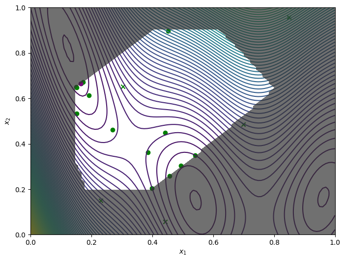
We obtain the final objective and constraint data using .try_get_final_datasets(). We can visualise how the optimizer performed by plotting all the acquired observations, along with the true function values and optima.
The crosses are the 5 initial points that were sampled from the entire search space. The green circles are the acquired observations by the optimizer. The purple circle is the best point found.
[9]:
from trieste.experimental.plotting import plot_bo_points, plot_function_2d


def plot_bo_results():
    dataset = result.try_get_final_dataset()
    query_points = dataset.query_points.numpy()
    observations = dataset.observations.numpy()

    _, ax = plot_function_2d(
        ScaledBranin.objective,
        constrained_search_space.lower,
        constrained_search_space.upper,
        contour=True,
        figsize=(8, 6),
    )

    plot_bo_points(
        query_points,
        ax[0, 0],
        num_initial_points,
        arg_min_idx,
        c_pass="green",
        c_best="purple",
    )

    ax[0, 0].contourf(
        xi,
        xj,
        constraint_values,
        levels=1,
        colors=[(0.2, 0.2, 0.2, 0.7), (1, 1, 1, 0)],
        zorder=2,
    )

    ax[0, 0].set_xlabel(r"$x_1$")
    ax[0, 0].set_ylabel(r"$x_2$")
    plt.show()


plot_bo_results()

Penalty method#
Acquisition function (penalty method)#
We recommend using the constrained optimization method above for cases where it can be used, as it should be more efficient. However there are setups when that method cannot be used, e.g. when using batches and some acquisition functions. For such cases, an alternative is to construct the standard expected constrained improvement (similar to the inequality-constraints notebook); except instead of using probability of feasibility with respect to the constraint model, we construct feasibility from the explicit input constraints. This feasibility is calculated by passing all the constraints residuals (to their respective limits) through a smooth step function and taking the product.
For this method, the FastConstraintsFeasibility class should be passed constraints via the search space. ExpectedConstrainedImprovement and BayesianOptimizer should be set up as usual without the constrained search space.
Note: this method penalises the expected improvement acquisition outside the feasible region. The optimizer uses the default scipy L-BFGS-B method to find the max of the acquistion function.
[10]:
from trieste.acquisition.function import (
    ExpectedConstrainedImprovement,
    FastConstraintsFeasibility,
)
from trieste.acquisition.rule import EfficientGlobalOptimization
from trieste.observer import OBJECTIVE

feas = FastConstraintsFeasibility(
    constrained_search_space
)  # Search space with constraints.
eci = ExpectedConstrainedImprovement(OBJECTIVE, feas.using(OBJECTIVE))

rule = EfficientGlobalOptimization(eci)
Run the optimization loop (penalty method)#
We can now run the optimization loop.
[11]:
# Note: use the search space without constraints for the penalty method.
bo = trieste.bayesian_optimizer.BayesianOptimizer(
    observer, unconstrained_search_space
)

result = bo.optimize(num_steps, initial_data, model, acquisition_rule=rule)
WARNING:tensorflow:5 out of the last 5 calls to <function fast_constraints_feasibility.<locals>.acquisition at 0x7fcf96746dd0> triggered tf.function retracing. Tracing is expensive and the excessive number of tracings could be due to (1) creating @tf.function repeatedly in a loop, (2) passing tensors with different shapes, (3) passing Python objects instead of tensors. For (1), please define your @tf.function outside of the loop. For (2), @tf.function has reduce_retracing=True option that can avoid unnecessary retracing. For (3), please refer to https://www.tensorflow.org/guide/function#controlling_retracing and https://www.tensorflow.org/api_docs/python/tf/function for  more details.
WARNING:tensorflow:6 out of the last 6 calls to <function fast_constraints_feasibility.<locals>.acquisition at 0x7fcf96746dd0> triggered tf.function retracing. Tracing is expensive and the excessive number of tracings could be due to (1) creating @tf.function repeatedly in a loop, (2) passing tensors with different shapes, (3) passing Python objects instead of tensors. For (1), please define your @tf.function outside of the loop. For (2), @tf.function has reduce_retracing=True option that can avoid unnecessary retracing. For (3), please refer to https://www.tensorflow.org/guide/function#controlling_retracing and https://www.tensorflow.org/api_docs/python/tf/function for  more details.
Optimization completed without errors
We can now get the best point found by the optimizer as before.
[12]:
query_point, observation, arg_min_idx = result.try_get_optimal_point()

print(f"query point: {query_point}")
print(f"observation: {observation}")
query point: [0.16545253 0.66525034]
observation: [-0.99877596]
Plot the results as before.
[13]:
plot_bo_results()