Batch Bayesian Optimization with Batch Expected Improvement, Local Penalization, Kriging Believer and GIBBON

Sometimes it is practically convenient to query several points at a time. This notebook demonstrates four ways to perfom batch Bayesian optimization with Trieste.

import numpy as np
import tensorflow as tf
from trieste.experimental.plotting import plot_acq_function_2d
import matplotlib.pyplot as plt
import trieste

np.random.seed(1234)
tf.random.set_seed(1234)

Describe the problem

In this example, we consider the same problem presented in our expected_improvement notebook, i.e. seeking the minimizer of the two-dimensional Branin function.

We begin our optimization after collecting five function evaluations from random locations in the search space.

from trieste.objectives import ScaledBranin
from trieste.objectives.utils import mk_observer
from trieste.space import Box

observer = mk_observer(ScaledBranin.objective)
search_space = Box([0, 0], [1, 1])

num_initial_points = 5
initial_query_points = search_space.sample(num_initial_points)
initial_data = observer(initial_query_points)

Surrogate model

Just like in purely sequential optimization, we fit a surrogate Gaussian process model to the initial data. The GPflow models cannot be used directly in our Bayesian optimization routines, so we build a GPflow’s GPR model using Trieste’s convenient model build function build_gpr and pass it to the GaussianProcessRegression wrapper. Note that we set the likelihood variance to a small number because we are dealing with a noise-free problem.

import gpflow
from trieste.models.gpflow import GaussianProcessRegression, build_gpr


gpflow_model = build_gpr(initial_data, search_space, likelihood_variance=1e-7)
model = GaussianProcessRegression(gpflow_model)

Batch acquisition functions.

To perform batch BO, we must define a batch acquisition function. Four batch acquisition functions supported in Trieste are BatchMonteCarloExpectedImprovement, LocalPenalization (see [GonzalezDHL16]), Fantasizer (see [GLRC10b]) and GIBBON (see [MLGR21]).

Although all these acquisition functions recommend batches of diverse query points, the batches are chosen in very different ways. BatchMonteCarloExpectedImprovement jointly allocates the batch of points as those with the largest expected improvement over our current best solution. In contrast, the LocalPenalization greedily builds the batch, sequentially adding the maximizers of the standard (non-batch) ExpectedImprovement function penalized around the current pending batch points. Fantasizer works similarly, but instead of penalizing the acquisition model, it iteratively updates the predictive equations after “fantasizing” obervations at the previously chosen query points. GIBBON also builds batches in a greedy manner but seeks batches that provide a large reduction in our uncertainty around the maximum value of the objective function.

In practice, BatchMonteCarloExpectedImprovement can be expected to have superior performance for small batches and dimension (batch_size<4) but scales poorly for larger batches, especially in high dimension. Fantasizer complexity scales cubically with the batch size, which also limits its use to small batches. LocalPenalization is computationally cheapest and may be the best fit for large batches.

Note that all these acquisition functions have controllable parameters. In particular, BatchMonteCarloExpectedImprovement is computed using a Monte-Carlo method (so it requires a sample_size), but uses a reparametrisation trick to make it deterministic. The LocalPenalization has parameters controlling the degree of penalization that must be estimated from a random sample of num_samples model predictions (we recommend at least 1_000 for each search space dimension). Similarly, GIBBON requires a grid_size parameter that controls its approximation accuracy (which should also be larger than 1_000 for each search space dimension). Fantasizer requires a method for “fantasizing” the observations, which can be done by sampling from the GP posterior or by using the GP posterior mean (a.k.a “kriging believer” heuristic, our default setup).

First, we collect the batch of ten points recommended by BatchMonteCarloExpectedImprovement …

from trieste.acquisition.function import BatchMonteCarloExpectedImprovement
from trieste.acquisition.rule import EfficientGlobalOptimization

monte_carlo_sample_size = 1000
batch_ei_acq = BatchMonteCarloExpectedImprovement(
    sample_size=monte_carlo_sample_size, jitter=1e-5
)
batch_size = 10
batch_ei_acq_rule = EfficientGlobalOptimization(  # type: ignore
    num_query_points=batch_size, builder=batch_ei_acq
)
points_chosen_by_batch_ei = batch_ei_acq_rule.acquire_single(
    search_space, model, dataset=initial_data
)

then we do the same with LocalPenalization …

from trieste.acquisition import LocalPenalization

sample_size = 2000
local_penalization_acq = LocalPenalization(
    search_space, num_samples=sample_size
)
local_penalization_acq_rule = EfficientGlobalOptimization(  # type: ignore
    num_query_points=batch_size, builder=local_penalization_acq
)
points_chosen_by_local_penalization = (
    local_penalization_acq_rule.acquire_single(
        search_space, model, dataset=initial_data
    )
)

then with Fantasizer …

from trieste.acquisition import Fantasizer

kriging_believer_acq = Fantasizer()
kriging_believer_acq_rule = EfficientGlobalOptimization(  # type: ignore
    num_query_points=batch_size, builder=kriging_believer_acq
)
points_chosen_by_kriging_believer = kriging_believer_acq_rule.acquire_single(
    search_space, model, dataset=initial_data
)

and finally we use GIBBON.

from trieste.acquisition.function import GIBBON

gibbon_acq = GIBBON(search_space, grid_size=sample_size)
gibbon_acq_rule = EfficientGlobalOptimization(  # type: ignore
    num_query_points=batch_size, builder=gibbon_acq
)
points_chosen_by_gibbon = gibbon_acq_rule.acquire_single(
    search_space, model, dataset=initial_data
)

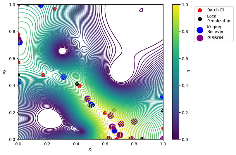
We can now visualize the batch of 10 points chosen by each of these methods overlayed on the standard ExpectedImprovement acquisition function. BatchMonteCarloExpectedImprovement and Fantasizer choose a more diverse set of points, whereas LocalPenalization and GIBBON focus evaluations in the most promising areas of the space.

from trieste.acquisition.function import ExpectedImprovement

# plot standard EI acquisition function
ei = ExpectedImprovement()
ei_acq_function = ei.prepare_acquisition_function(model, dataset=initial_data)
plot_acq_function_2d(
    ei_acq_function,
    [0, 0],
    [1, 1],
    contour=True,
)

plt.scatter(
    points_chosen_by_batch_ei[:, 0],
    points_chosen_by_batch_ei[:, 1],
    color="red",
    lw=5,
    label="Batch-EI",
    marker="*",
    zorder=1,
)
plt.scatter(
    points_chosen_by_local_penalization[:, 0],
    points_chosen_by_local_penalization[:, 1],
    color="black",
    lw=10,
    label="Local \nPenalization",
    marker="+",
)
plt.scatter(
    points_chosen_by_kriging_believer[:, 0],
    points_chosen_by_kriging_believer[:, 1],
    color="blue",
    lw=10,
    label="Kriging \nBeliever",
    marker="o",
)
plt.scatter(
    points_chosen_by_gibbon[:, 0],
    points_chosen_by_gibbon[:, 1],
    color="purple",
    lw=10,
    label="GIBBON",
    marker="X",
)


plt.legend(bbox_to_anchor=(1.2, 1), loc="upper left")
plt.xlabel(r"$x_1$")
plt.ylabel(r"$x_2$")
cbar = plt.colorbar()
cbar.set_label("EI", rotation=270)

/opt/hostedtoolcache/Python/3.10.12/x64/lib/python3.10/site-packages/matplotlib/_mathtext.py:1880: UserWarning: warn_name_set_on_empty_Forward: setting results name 'sym' on Forward expression that has no contained expression
  - p.placeable("sym"))
/opt/hostedtoolcache/Python/3.10.12/x64/lib/python3.10/site-packages/matplotlib/_mathtext.py:1885: UserWarning: warn_ungrouped_named_tokens_in_collection: setting results name 'name' on ZeroOrMore expression collides with 'name' on contained expression
  "{" + ZeroOrMore(p.simple | p.unknown_symbol)("name") + "}")

Run the batch optimization loop

We can now run a batch Bayesian optimization loop by defining a BayesianOptimizer with one of our batch acquisition functions.

We reuse the same EfficientGlobalOptimization rule as in the purely sequential case, however we pass in one of batch acquisition functions and set num_query_points>1.

We’ll run each method for ten steps for batches of three points.

First we run ten steps of BatchMonteCarloExpectedImprovement …

bo = trieste.bayesian_optimizer.BayesianOptimizer(observer, search_space)

batch_ei_rule = EfficientGlobalOptimization(  # type: ignore
    num_query_points=3, builder=batch_ei_acq
)
num_steps = 10
qei_result = bo.optimize(
    num_steps, initial_data, model, acquisition_rule=batch_ei_rule
)

Optimization completed without errors

then we repeat the same optimization with LocalPenalization…

local_penalization_rule = EfficientGlobalOptimization(  # type: ignore
    num_query_points=3, builder=local_penalization_acq
)
local_penalization_result = bo.optimize(
    num_steps, initial_data, model, acquisition_rule=local_penalization_rule
)

Optimization completed without errors

then with Fantasizer…

kriging_believer_rule = EfficientGlobalOptimization(  # type: ignore
    num_query_points=3, builder=kriging_believer_acq
)
kriging_believer_result = bo.optimize(
    num_steps, initial_data, model, acquisition_rule=kriging_believer_rule
)

Optimization completed without errors

and finally with the GIBBON acquisition function.

gibbon_rule = EfficientGlobalOptimization(  # type: ignore
    num_query_points=3, builder=gibbon_acq
)
gibbon_result = bo.optimize(
    num_steps, initial_data, model, acquisition_rule=gibbon_rule
)

Optimization completed without errors

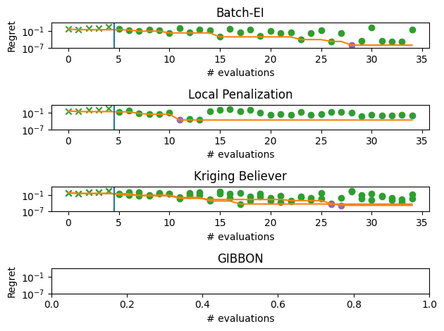
We can visualize the performance of each of these methods by plotting the trajectory of the regret (suboptimality) of the best observed solution as the optimization progresses. We denote this trajectory with the orange line, the start of the optimization loop with the blue line and the best overall point as a purple dot.

For this particular problem (and random seed), we see that GIBBON provides the fastest initial optimization but all methods have overall a roughly similar performance.

from trieste.experimental.plotting import plot_regret

qei_observations = (
    qei_result.try_get_final_dataset().observations - ScaledBranin.minimum
)
qei_min_idx = tf.squeeze(tf.argmin(qei_observations, axis=0))
local_penalization_observations = (
    local_penalization_result.try_get_final_dataset().observations
    - ScaledBranin.minimum
)
local_penalization_min_idx = tf.squeeze(
    tf.argmin(local_penalization_observations, axis=0)
)
kriging_believer_observations = (
    kriging_believer_result.try_get_final_dataset().observations
    - ScaledBranin.minimum
)
kriging_believer_min_idx = tf.squeeze(
    tf.argmin(kriging_believer_observations, axis=0)
)
gibbon_observations = (
    gibbon_result.try_get_final_dataset().observations - ScaledBranin.minimum
)
gibbon_min_idx = tf.squeeze(tf.argmin(gibbon_observations, axis=0))


fig, ax = plt.subplots(4, 1)
plot_regret(qei_observations.numpy(), ax[0], num_init=5, idx_best=qei_min_idx)
ax[0].set_yscale("log")
ax[0].set_ylabel("Regret")
ax[0].set_ylim(0.0000001, 100)
ax[0].set_xlabel("# evaluations")
ax[0].set_title("Batch-EI")

plot_regret(
    local_penalization_observations.numpy(),
    ax[1],
    num_init=5,
    idx_best=local_penalization_min_idx,
)
ax[1].set_yscale("log")
ax[1].set_xlabel("# evaluations")
ax[1].set_ylim(0.0000001, 100)
ax[1].set_title("Local Penalization")

plot_regret(
    kriging_believer_observations.numpy(),
    ax[2],
    num_init=5,
    idx_best=kriging_believer_min_idx,
)
ax[2].set_yscale("log")
ax[2].set_xlabel("# evaluations")
ax[2].set_ylim(0.0000001, 100)
ax[2].set_title("Kriging Believer")

plot_regret(
    gibbon_observations.numpy(), ax[2], num_init=5, idx_best=gibbon_min_idx
)
ax[3].set_yscale("log")
ax[3].set_ylabel("Regret")
ax[3].set_ylim(0.0000001, 100)
ax[3].set_xlabel("# evaluations")
ax[3].set_title("GIBBON")

fig.tight_layout()

LICENSE

Apache License 2.0