Batch HSRI Tutorial

Batch Hypervolume Sharpe Ratio Indicator (qHSRI) is a method proposed by Binois et al. (see [BCO21]) for picking a batch of query points during Bayesian Optimisation. It makes use of the Sharpe Ratio, a portfolio selection method used in investment selection to carefully balance risk and reward.

This tutorial will first cover the main points of how the Trieste implementation of qHSRI works under the hood, and then demonstrate how to use the trieste.acquisition.rule.BatchHypervolumeRatioIndicator acquisition rule.

Some of the dependencies for BatchHypervolumeRatioIndicator are not included in Trieste by default, and instead can be installed via pip install trieste[qhsri].

First we will set up our problem and get our initial datapoints. For this walkthrough we will use the noiseless scaled Branin objective.

import tensorflow as tf
import matplotlib.pyplot as plt

from trieste.objectives import ScaledBranin
from trieste.objectives.utils import mk_observer
from trieste.space import Box

tf.random.set_seed(1)

# Create the observer
observer = mk_observer(ScaledBranin.objective)

# Define Search space
search_space = Box([0, 0], [1, 1])

# Set initial number of query points
num_initial_points = 5
initial_query_points = search_space.sample(num_initial_points)
initial_data = observer(initial_query_points)

We can now fit a GP to our initial data.

from trieste.models.gpflow import GaussianProcessRegression, build_gpr

# Set up model
gpflow_model = build_gpr(initial_data, search_space, likelihood_variance=1e-7)
model = GaussianProcessRegression(gpflow_model)

Now consider how we might want to select a batch of \(q\) query points to observe. It would be useful for some of these to be “safe bets” that we think are very likely to provide good values (i.e low predicted mean). It would also be valuable for some of these to be sampling parts of the space that we have no idea what the expected observed value is (i.e. high variance). This problem is very similar to that encountered in building finance portfolios, where you want a mix of high risk/high reward and low risk/low reward assets. You would also want to know how much of your total capital to invest in each asset.

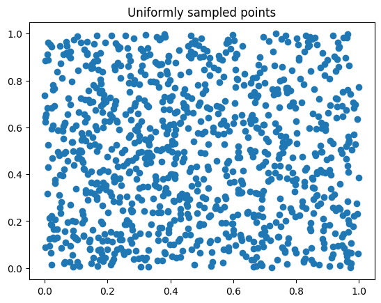
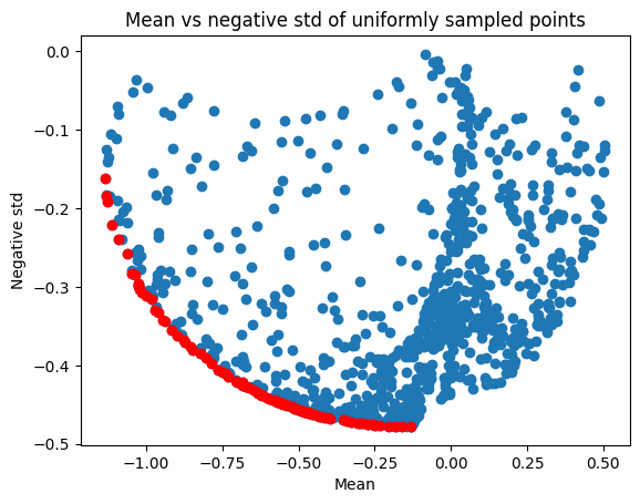
To visualise the different trade-offs, we can sample from the input space, compute the predictive mean and variance at those locations, and plot the mean against minus the standard deviation (so that both quantities need to be minimised)

uniform_points = search_space.sample(1000)
uniform_pts_mean, uniform_pts_var = model.predict(uniform_points)
uniform_pts_std = -tf.sqrt(uniform_pts_var)

plt.scatter(uniform_points[:, 0], uniform_points[:, 1])
plt.title("Uniformly sampled points")
plt.show()
plt.close()

plt.scatter(uniform_pts_mean, uniform_pts_std)
plt.title("Mean vs negative std of uniformly sampled points")
plt.xlabel("Mean")
plt.ylabel("Negative std")
plt.show()

Since we only want the best points in terms of the risk-reward tradeoff, we can remove all the points that are not optimal in the Pareto sense, i.e. the points that are dominated by another point. A point a is dominated by another point b if b.mean <= a.mean and b.std >= a.std.

There is a function in trieste that lets us calculate this non-dominated set. Let’s find the non-dominated points and plot them on the above chart.

from trieste.acquisition.multi_objective.dominance import non_dominated

uniform_non_dominated = non_dominated(
    tf.concat([uniform_pts_mean, uniform_pts_std], axis=1)
)[0]

plt.scatter(uniform_pts_mean, uniform_pts_std)
plt.scatter(uniform_non_dominated[:, 0], uniform_non_dominated[:, 1], c="r")
plt.title("Mean vs negative std of uniformly sampled points")
plt.xlabel("Mean")
plt.ylabel("Negative std")
plt.show()

print(f"There are {len(uniform_non_dominated)} non-dominated points")

There are 93 non-dominated points

We can see that there’s only a few non-dominated points to choose from the select the next batch. This set of non-dominated points is the Pareto front in the optimisation task of minimising mean and maximising standard deviation.

This means we can improve on this by using optimisation rather than random sampling to pick the points that we will select our batch from. In trieste we use the NSGA-II multi-objective optimisation method from the pymoo library to find the Pareto front.

The BatchHypervolumeSharpeRatioIndicator acquisition rule makes use of the _MeanStdTradeoff class, which expresses the optimisation problem in the pymoo framework. Pymoo is then used to run the optimisation.

NSGA-II is a genetic algorithm, and so we need to define a population size and number of generations.

import numpy as np
from trieste.acquisition.rule import _MeanStdTradeoff
from pymoo.algorithms.moo.nsga2 import NSGA2
from pymoo.optimize import minimize

problem = _MeanStdTradeoff(model, search_space)
algorithm = NSGA2(pop_size=500)
result = minimize(problem, algorithm, ("n_gen", 200), seed=1, verbose=False)
optimised_points, optimised_mean_std = result.X, result.F

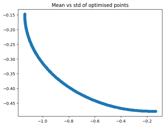
Now we can plot the points that have been optimised for mean and standard deviation, and their means and stds.

plt.scatter(result.X[:, 0], result.X[:, 1])
plt.title("Points optimised for mean and std")
plt.show()

plt.scatter(result.F[:, 0], result.F[:, 1])
plt.title("Mean vs std of optimised points")
plt.show()

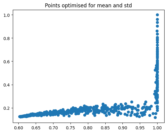
We can check the non-dominated points again, and see that the outcome of NSGA-II is much better than the randomly sampled ones.

optimised_non_dominated = non_dominated(result.F)[0]
plt.scatter(result.F[:, 0], result.F[:, 1])
plt.scatter(optimised_non_dominated[:, 0], optimised_non_dominated[:, 1], c="r")
plt.show()
print(f"There are {len(optimised_non_dominated)} non-dominated points")

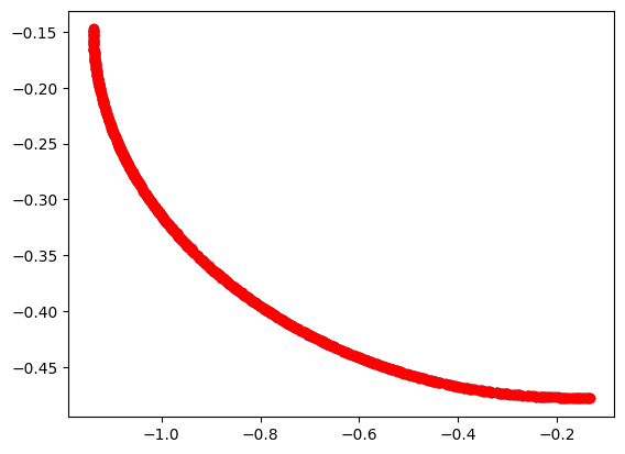
There are 500 non-dominated points

The Sharpe ratio is used to get an optimal mix of low mean and high standard deviation points from this Pareto front, so that these can then be observed.

A portfolio with the maximum Sharpe ratio is defined as:

\[\max_{x \in [0,1]^n} h(x) = {{r^{T}x-r_{f}} \over {\sqrt{x^{T}Qx}}} \;\;\; s.t \sum^{n}_{i=1}x_i = 1\]

where \(x_i\) are weights for each asset \(i\), \(r_i\) is the expected return of asset \(i\) and \(Q_{i,j}\) is the covariance of assets \(i\) and \(j\). \(r_f\) is a risk free asset, and we will assume this does not exist in this case. Note that weighting assets with high expected rewards will increase the Sharpe ratio, as will weighting assets with low covariance.

This problem can be converted into a quadratic programming problem and solved to give a diverse sample from the Pareto front.

The trieste.acquisition.multi_objective.Pareto class has a sample_diverse_subset method that implements this.

from trieste.acquisition.multi_objective import Pareto

# Since we've already ensured the set is non-dominated we don't need to repeat this
front = Pareto(optimised_non_dominated, already_non_dominated=True)

sampled_points, _ = front.sample_diverse_subset(
    sample_size=5, allow_repeats=False
)

Now we can see which points we selected from the Pareto front

plt.scatter(
    optimised_non_dominated[:, 0],
    optimised_non_dominated[:, 1],
    label="Pareto front",
)
plt.scatter(sampled_points[:, 0], sampled_points[:, 1], label="selected points")
plt.legend()
plt.title("Pareto front and selected points for observation")
plt.show()

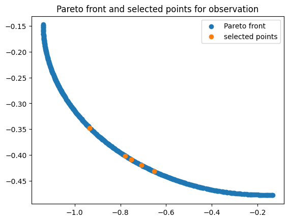
These points can then be observed and the model updated. This aquisition method has been implemented in trieste as an acquisition rule, trieste.acquisition.rule.BatchHypervolumeRatioIndicator.

Using the Acqusition rule for Bayesian Optimisation

The BatchHypervolumeRatioIndicator can be used in the same way as other batch acquisition rules. We set up the problem as before, and then run optimize with the BatchHypervolumeRatioIndicator rule.

from trieste.bayesian_optimizer import BayesianOptimizer
from trieste.acquisition.rule import BatchHypervolumeSharpeRatioIndicator

# Create observer
observer = mk_observer(ScaledBranin.objective)

# Define Search space
search_space = Box([0, 0], [1, 1])

# Set initial number of query points
num_initial_points = 5
initial_query_points = search_space.sample(num_initial_points)
initial_data = observer(initial_query_points)

from trieste.models.gpflow import GaussianProcessRegression, build_gpr

# Set up model
gpflow_model = build_gpr(initial_data, search_space, likelihood_variance=1e-3)
model = GaussianProcessRegression(gpflow_model)

bo = BayesianOptimizer(observer=observer, search_space=search_space)

results = bo.optimize(
    acquisition_rule=BatchHypervolumeSharpeRatioIndicator(num_query_points=10),
    num_steps=8,
    datasets=initial_data,
    models=model,
)

Optimization completed without errors

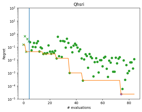
We can now plot the regret of the observations, and see that the regret has decreased from the initial sample.

from trieste.experimental.plotting import plot_regret

observations = (
    results.try_get_final_dataset().observations - ScaledBranin.minimum
)

min_idx = tf.squeeze(tf.argmin(observations, axis=0))
min_regret = tf.reduce_min(observations)

fig, ax = plt.subplots(1, 1)
plot_regret(observations.numpy(), ax, num_init=5, idx_best=min_idx)
ax.set_yscale("log")
ax.set_ylabel("Regret")
ax.set_ylim(0.00001, 100)
ax.set_xlabel("# evaluations")
ax.set_title("Qhsri")
plt.show()

/opt/hostedtoolcache/Python/3.10.12/x64/lib/python3.10/site-packages/matplotlib/_mathtext.py:1880: UserWarning: warn_name_set_on_empty_Forward: setting results name 'sym' on Forward expression that has no contained expression
  - p.placeable("sym"))
/opt/hostedtoolcache/Python/3.10.12/x64/lib/python3.10/site-packages/matplotlib/_mathtext.py:1885: UserWarning: warn_ungrouped_named_tokens_in_collection: setting results name 'name' on ZeroOrMore expression collides with 'name' on contained expression
  "{" + ZeroOrMore(p.simple | p.unknown_symbol)("name") + "}")