Using deep Gaussian processes with GPflux for Bayesian optimization.

import numpy as np
import tensorflow as tf

np.random.seed(1794)
tf.random.set_seed(1794)

Describe the problem

In this notebook, we show how to use deep Gaussian processes (DGPs) for Bayesian optimization using Trieste and GPflux. DGPs may be better for modeling non-stationary objective functions than standard GP surrogates, as discussed in [DKvdH+17, HBB+19].

In this example, we look to find the minimum value of the two- and five-dimensional Michalewicz functions over the hypercubes \([0, pi]^2\)/\([0, pi]^5\). We compare a two-layer DGP model with GPR, using Thompson sampling for both.

The Michalewicz functions are highly non-stationary and have a global minimum that’s hard to find, so DGPs might be more suitable than standard GPs, which may struggle because they typically have stationary kernels that cannot easily model non-stationarities.

import gpflow
from trieste.objectives import Michalewicz2, Michalewicz5
from trieste.objectives.utils import mk_observer
from trieste.experimental.plotting import plot_function_plotly

function = Michalewicz2.objective
F_MINIMIZER = Michalewicz2.minimum

search_space = Michalewicz2.search_space

fig = plot_function_plotly(function, search_space.lower, search_space.upper)
fig.show()

Sample the observer over the search space

We set up the observer as usual, using Sobol sampling to sample the initial points.

import trieste

observer = mk_observer(function)

num_initial_points = 20
num_steps = 20
initial_query_points = search_space.sample_sobol(num_initial_points)
initial_data = observer(initial_query_points)

Model the objective function

The Bayesian optimization procedure estimates the next best points to query by using a probabilistic model of the objective. We’ll use a two layer deep Gaussian process (DGP), built using GPflux. We also compare to a (shallow) GP.

Since DGPs can be hard to build, Trieste provides some basic architectures: here we use the build_vanilla_deep_gp function which returns a GPflux model of DeepGP class. As with other models (e.g. GPflow), we cannot use it directly in Bayesian optimization routines, we need to pass it through an appropriate wrapper, DeepGaussianProcess wrapper in this case. Additionally, since the GPflux interface does not currently support copying DGP architectures, if we wish to have the Bayesian optimizer track the model state, we need to pass in the DGP as a callable closure so that the architecture can be recreated when required (alternatively, we can set set_state=False on the optimize call).

A few other useful notes regarding building a DGP model: The DGP model requires us to specify the number of inducing points, as we don’t have the true posterior. To train the model we have to use a stochastic optimizer; Adam is used by default, but we can use other stochastic optimizers from TensorFlow. GPflux allows us to use the Keras fit method, which makes optimizing a lot easier - this method is used in the background for training the model.

from functools import partial

from trieste.models.gpflux import DeepGaussianProcess, build_vanilla_deep_gp


def build_dgp_model(data, search_space):
    dgp = partial(
        build_vanilla_deep_gp,
        data,
        search_space,
        2,
        100,
        likelihood_variance=1e-5,
        trainable_likelihood=False,
    )
    return DeepGaussianProcess(dgp)


dgp_model = build_dgp_model(initial_data, search_space)

WARNING:tensorflow:From /opt/hostedtoolcache/Python/3.10.12/x64/lib/python3.10/site-packages/tensorflow_probability/python/distributions/distribution.py:342: calling MultivariateNormalDiag.__init__ (from tensorflow_probability.python.distributions.mvn_diag) with scale_identity_multiplier is deprecated and will be removed after 2020-01-01.
Instructions for updating:
`scale_identity_multiplier` is deprecated; please combine it into `scale_diag` directly instead.

Run the optimization loop

We can now run the Bayesian optimization loop by defining a BayesianOptimizer and calling its optimize method.

The optimizer uses an acquisition rule to choose where in the search space to try on each optimization step. We’ll start by using Thompson sampling.

We’ll run the optimizer for twenty steps. Note: this may take a while!

from trieste.acquisition.rule import DiscreteThompsonSampling

bo = trieste.bayesian_optimizer.BayesianOptimizer(observer, search_space)
grid_size = 1000
acquisition_rule = DiscreteThompsonSampling(grid_size, 1)

dgp_result = bo.optimize(
    num_steps,
    initial_data,
    dgp_model,
    acquisition_rule=acquisition_rule,
)
dgp_dataset = dgp_result.try_get_final_dataset()

WARNING:tensorflow:5 out of the last 5 calls to <function dgp_feature_decomposition_trajectory.__call__ at 0x7f38f14e9360> triggered tf.function retracing. Tracing is expensive and the excessive number of tracings could be due to (1) creating @tf.function repeatedly in a loop, (2) passing tensors with different shapes, (3) passing Python objects instead of tensors. For (1), please define your @tf.function outside of the loop. For (2), @tf.function has reduce_retracing=True option that can avoid unnecessary retracing. For (3), please refer to https://www.tensorflow.org/guide/function#controlling_retracing and https://www.tensorflow.org/api_docs/python/tf/function for  more details.
WARNING:tensorflow:6 out of the last 6 calls to <function dgp_feature_decomposition_trajectory.__call__ at 0x7f38f12bf520> triggered tf.function retracing. Tracing is expensive and the excessive number of tracings could be due to (1) creating @tf.function repeatedly in a loop, (2) passing tensors with different shapes, (3) passing Python objects instead of tensors. For (1), please define your @tf.function outside of the loop. For (2), @tf.function has reduce_retracing=True option that can avoid unnecessary retracing. For (3), please refer to https://www.tensorflow.org/guide/function#controlling_retracing and https://www.tensorflow.org/api_docs/python/tf/function for  more details.
Optimization completed without errors

Explore the results

We can now get the best point found by the optimizer. Note this isn’t necessarily the point that was last evaluated.

dgp_query_points = dgp_dataset.query_points.numpy()
dgp_observations = dgp_dataset.observations.numpy()

dgp_arg_min_idx = tf.squeeze(tf.argmin(dgp_observations, axis=0))

print(f"query point: {dgp_query_points[dgp_arg_min_idx, :]}")
print(f"observation: {dgp_observations[dgp_arg_min_idx, :]}")

query point: [2.19634826 1.5960335 ]
observation: [-1.77473032]

We can visualise how the optimizer performed as a three-dimensional plot

from trieste.experimental.plotting import add_bo_points_plotly

fig = plot_function_plotly(
    function, search_space.lower, search_space.upper, alpha=0.5
)

fig = add_bo_points_plotly(
    x=dgp_query_points[:, 0],
    y=dgp_query_points[:, 1],
    z=dgp_observations[:, 0],
    num_init=num_initial_points,
    idx_best=dgp_arg_min_idx,
    fig=fig,
)
fig.show()

We can visualise the model over the objective function by plotting the mean and 95% confidence intervals of its predictive distribution. Note that the DGP model is able to model the local structure of the true objective function.

import matplotlib.pyplot as plt
from trieste.experimental.plotting import (
    plot_regret,
    plot_model_predictions_plotly,
)

fig = plot_model_predictions_plotly(
    dgp_result.try_get_final_model(),
    search_space.lower,
    search_space.upper,
    num_samples=100,
)

fig = add_bo_points_plotly(
    x=dgp_query_points[:, 0],
    y=dgp_query_points[:, 1],
    z=dgp_observations[:, 0],
    num_init=num_initial_points,
    idx_best=dgp_arg_min_idx,
    fig=fig,
    figrow=1,
    figcol=1,
)
fig.show()

We now compare to a GP model with priors over the hyperparameters. We do not expect this to do as well because GP models cannot deal with non-stationary functions well.

import gpflow
import tensorflow_probability as tfp

from trieste.models.gpflow import GaussianProcessRegression, build_gpr

gpflow_model = build_gpr(initial_data, search_space, likelihood_variance=1e-7)
gp_model = GaussianProcessRegression(gpflow_model)

bo = trieste.bayesian_optimizer.BayesianOptimizer(observer, search_space)

result = bo.optimize(
    num_steps,
    initial_data,
    gp_model,
    acquisition_rule=acquisition_rule,
)
gp_dataset = result.try_get_final_dataset()

gp_query_points = gp_dataset.query_points.numpy()
gp_observations = gp_dataset.observations.numpy()

gp_arg_min_idx = tf.squeeze(tf.argmin(gp_observations, axis=0))

print(f"query point: {gp_query_points[gp_arg_min_idx, :]}")
print(f"observation: {gp_observations[gp_arg_min_idx, :]}")

fig = plot_model_predictions_plotly(
    result.try_get_final_model(),
    search_space.lower,
    search_space.upper,
)

fig = add_bo_points_plotly(
    x=gp_query_points[:, 0],
    y=gp_query_points[:, 1],
    z=gp_observations[:, 0],
    num_init=num_initial_points,
    idx_best=gp_arg_min_idx,
    fig=fig,
    figrow=1,
    figcol=1,
)
fig.show()

Optimization completed without errors
query point: [2.20267349 1.57829009]
observation: [-1.79901999]

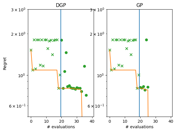
We see that the DGP model does a much better job at understanding the structure of the function. The standard Gaussian process model has a large signal variance and small lengthscales, which do not result in a good model of the true objective. On the other hand, the DGP model is at least able to infer the local structure around the observations.

We can also plot the regret curves of the two models side-by-side.

gp_suboptimality = gp_observations - F_MINIMIZER.numpy()
dgp_suboptimality = dgp_observations - F_MINIMIZER.numpy()

_, ax = plt.subplots(1, 2)
plot_regret(
    dgp_suboptimality,
    ax[0],
    num_init=num_initial_points,
    idx_best=dgp_arg_min_idx,
)
plot_regret(
    gp_suboptimality,
    ax[1],
    num_init=num_initial_points,
    idx_best=gp_arg_min_idx,
)

ax[0].set_yscale("log")
ax[0].set_ylabel("Regret")
ax[0].set_ylim(0.5, 3)
ax[0].set_xlabel("# evaluations")
ax[0].set_title("DGP")

ax[1].set_title("GP")
ax[1].set_yscale("log")
ax[1].set_ylim(0.5, 3)
ax[1].set_xlabel("# evaluations")

Text(0.5, 0, '# evaluations')

/opt/hostedtoolcache/Python/3.10.12/x64/lib/python3.10/site-packages/matplotlib/_mathtext.py:1880: UserWarning:

warn_name_set_on_empty_Forward: setting results name 'sym' on Forward expression that has no contained expression

/opt/hostedtoolcache/Python/3.10.12/x64/lib/python3.10/site-packages/matplotlib/_mathtext.py:1885: UserWarning:

warn_ungrouped_named_tokens_in_collection: setting results name 'name' on ZeroOrMore expression collides with 'name' on contained expression

We might also expect that the DGP model will do better on higher dimensional data. We explore this by testing a higher-dimensional version of the Michalewicz dataset.

Set up the problem.

function = Michalewicz5.objective
F_MINIMIZER = Michalewicz5.minimum

search_space = Michalewicz5.search_space

observer = mk_observer(function)

num_initial_points = 50
num_steps = 50
initial_query_points = search_space.sample_sobol(num_initial_points)
initial_data = observer(initial_query_points)

Build the DGP model and run the Bayes opt loop.

dgp_model = build_dgp_model(initial_data, search_space)

bo = trieste.bayesian_optimizer.BayesianOptimizer(observer, search_space)
acquisition_rule = DiscreteThompsonSampling(grid_size, 1)

dgp_result = bo.optimize(
    num_steps,
    initial_data,
    dgp_model,
    acquisition_rule=acquisition_rule,
)
dgp_dataset = dgp_result.try_get_final_dataset()

dgp_query_points = dgp_dataset.query_points.numpy()
dgp_observations = dgp_dataset.observations.numpy()

dgp_arg_min_idx = tf.squeeze(tf.argmin(dgp_observations, axis=0))

print(f"query point: {dgp_query_points[dgp_arg_min_idx, :]}")
print(f"observation: {dgp_observations[dgp_arg_min_idx, :]}")

dgp_suboptimality = dgp_observations - F_MINIMIZER.numpy()

Optimization completed without errors
query point: [1.88377634 1.47870954 2.42776428 1.96987102 0.97230414]
observation: [-2.18461384]

Repeat the above for the GP model.

gpflow_model = build_gpr(initial_data, search_space, likelihood_variance=1e-7)
gp_model = GaussianProcessRegression(gpflow_model)

bo = trieste.bayesian_optimizer.BayesianOptimizer(observer, search_space)

result = bo.optimize(
    num_steps,
    initial_data,
    gp_model,
    acquisition_rule=acquisition_rule,
)
gp_dataset = result.try_get_final_dataset()

gp_query_points = gp_dataset.query_points.numpy()
gp_observations = gp_dataset.observations.numpy()

gp_arg_min_idx = tf.squeeze(tf.argmin(gp_observations, axis=0))

print(f"query point: {gp_query_points[gp_arg_min_idx, :]}")
print(f"observation: {gp_observations[gp_arg_min_idx, :]}")

gp_suboptimality = gp_observations - F_MINIMIZER.numpy()

Optimization completed without errors
query point: [2.39002255 1.53970234 2.21992787 1.74455962 1.76705085]
observation: [-2.62917686]

Plot the regret.

_, ax = plt.subplots(1, 2)
plot_regret(
    dgp_suboptimality,
    ax[0],
    num_init=num_initial_points,
    idx_best=dgp_arg_min_idx,
)
plot_regret(
    gp_suboptimality,
    ax[1],
    num_init=num_initial_points,
    idx_best=gp_arg_min_idx,
)

ax[0].set_yscale("log")
ax[0].set_ylabel("Regret")
ax[0].set_ylim(1.5, 6)
ax[0].set_xlabel("# evaluations")
ax[0].set_title("DGP")

ax[1].set_title("GP")
ax[1].set_yscale("log")
ax[1].set_ylim(1.5, 6)
ax[1].set_xlabel("# evaluations")

Text(0.5, 0, '# evaluations')

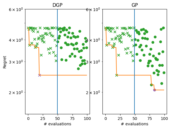
While still far from the optimum, it is considerably better than the GP.

LICENSE

Apache License 2.0