Introduction to GPflux

In this notebook we cover the basics of Deep Gaussian processes (DGPs) [DL13] with GPflux. We assume that the reader is familiar with the concepts of Gaussian processes and Deep GPs (see [RW06, vdWDJ+20] for an in-depth overview).

import matplotlib.pyplot as plt
import numpy as np
import pandas as pd
import tensorflow as tf

tf.get_logger().setLevel("INFO")

2024-01-08 14:39:50.607849: I tensorflow/tsl/cuda/cudart_stub.cc:28] Could not find cuda drivers on your machine, GPU will not be used.
2024-01-08 14:39:50.638097: I tensorflow/tsl/cuda/cudart_stub.cc:28] Could not find cuda drivers on your machine, GPU will not be used.
2024-01-08 14:39:50.638740: I tensorflow/core/platform/cpu_feature_guard.cc:182] This TensorFlow binary is optimized to use available CPU instructions in performance-critical operations.
To enable the following instructions: AVX2 FMA, in other operations, rebuild TensorFlow with the appropriate compiler flags.

2024-01-08 14:39:51.319003: W tensorflow/compiler/tf2tensorrt/utils/py_utils.cc:38] TF-TRT Warning: Could not find TensorRT

The motorcycle dataset

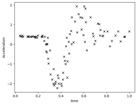
We are going to model a one-dimensional dataset containing observations from a simulated motorcycle accident, used to test crash helmets [1]. The dataset has many interesting properties that we can use to showcase the power of DGPs as opposed to shallow (that is, single layer) GP models.

def motorcycle_data():
    """Return inputs and outputs for the motorcycle dataset. We normalise the outputs."""
    df = pd.read_csv("./data/motor.csv", index_col=0)
    X, Y = df["times"].values.reshape(-1, 1), df["accel"].values.reshape(-1, 1)
    Y = (Y - Y.mean()) / Y.std()
    X /= X.max()
    return X, Y


X, Y = motorcycle_data()
plt.plot(X, Y, "kx")
plt.xlabel("time")
plt.ylabel("Acceleration")

Text(0, 0.5, 'Acceleration')

Single-layer GP

We start this introduction by building a single-layer GP using GPflux. However, you’ll notice that we rely a lot on GPflow objects to build our GPflux model. This is a conscious decision. GPflow contains well-tested and stable implementations of key GP building blocks, such as kernels, likelihoods, inducing variables, mean functions, and so on. By relying on GPflow for these elements, we can keep the GPflux code lean and focused on what is important for building deep GP models.

We are going to build a Sparse Variational Gaussian process (SVGP), for which we refer to [vdWDJ+20] or [LDJD20] for an in-depth overview.

We start by importing gpflow and gpflux, and then create a kernel and inducing variable. Both are GPflow objects. We pass both objects to a GPLayer which will represent a single GP layer in our deep GP. We also need to specify the total number of datapoints and the number of outputs.

import gpflow
import gpflux

num_data = len(X)
num_inducing = 10
output_dim = Y.shape[1]

kernel = gpflow.kernels.SquaredExponential()
inducing_variable = gpflow.inducing_variables.InducingPoints(
    np.linspace(X.min(), X.max(), num_inducing).reshape(-1, 1)
)
gp_layer = gpflux.layers.GPLayer(
    kernel, inducing_variable, num_data=num_data, num_latent_gps=output_dim
)

/home/runner/work/GPflux/GPflux/gpflux/layers/gp_layer.py:175: UserWarning: Beware, no mean function was specified in the construction of the `GPLayer` so the default `gpflow.mean_functions.Identity` is being used. This mean function will only work if the input dimensionality matches the number of latent Gaussian processes in the layer.
  warnings.warn(
/home/runner/work/GPflux/GPflux/gpflux/layers/gp_layer.py:198: UserWarning: Could not verify the compatibility of the `kernel`, `inducing_variable` and `mean_function`. We advise using `gpflux.helpers.construct_*` to create compatible kernels and inducing variables. As `num_latent_gps=1` has been specified explicitly, this will be used to create the `q_mu` and `q_sqrt` parameters.
  warnings.warn(

We now create a LikelihoodLayer which encapsulates a Likelihood from GPflow. The likelihood layer is responsible for computing the variational expectation in the objective, and for dealing with our likelihood distribution \(p(y | f)\). Other typical likelihoods are Softmax, RobustMax, and Bernoulli. Because we are dealing with the simple case of regression in this notebook, we use the Gaussian likelihood.

likelihood_layer = gpflux.layers.LikelihoodLayer(gpflow.likelihoods.Gaussian(0.1))

/tmp/ipykernel_3296/153007595.py:1: DeprecationWarning: Call to deprecated class TrackableLayer. (GPflux's `TrackableLayer` was prior to TF2.5 used to collect GPflow variables in subclassed layers. As of TF 2.5, `tf.Module` supports this natively and there is no need for `TrackableLayer` anymore. It will be removed in GPflux version `1.0.0`.)
  likelihood_layer = gpflux.layers.LikelihoodLayer(gpflow.likelihoods.Gaussian(0.1))

We now pass our GP layer and likelihood layer into a GPflux DeepGP model. The DeepGP class is a specialisation of the Keras Model where we’ve added a few helper methods such as predict_f, predict_y, and elbo. By relying on Keras, we hope that users will have an easy time familiarising themselves with the GPflux API. Our DeepGP model has the same public API calls: fit, predict, evaluate, and so on.

single_layer_dgp = gpflux.models.DeepGP([gp_layer], likelihood_layer)
model = single_layer_dgp.as_training_model()
model.compile(tf.optimizers.Adam(0.01))

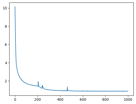
We train the model by calling fit. Keras handles minibatching the data, and keeps track of our loss during training.

history = model.fit({"inputs": X, "targets": Y}, epochs=int(1e3), verbose=0)
plt.plot(history.history["loss"])

[<matplotlib.lines.Line2D at 0x7f63cc0d6d90>]

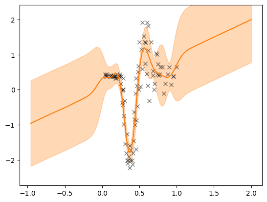
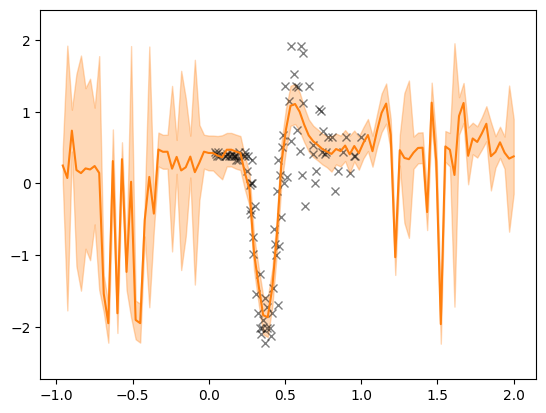
We can now visualise the fit. We clearly see that a single layer GP with a simple stationary kernel has trouble fitting this dataset.

def plot(model, X, Y, ax=None):
    if ax is None:
        fig, ax = plt.subplots()

    a = 1.0
    N_test = 100
    X_test = np.linspace(X.min() - a, X.max() + a, N_test).reshape(-1, 1)
    out = model(X_test)

    mu = out.f_mean.numpy().squeeze()
    var = out.f_var.numpy().squeeze()
    X_test = X_test.squeeze()
    lower = mu - 2 * np.sqrt(var)
    upper = mu + 2 * np.sqrt(var)

    ax.set_ylim(Y.min() - 0.5, Y.max() + 0.5)
    ax.plot(X, Y, "kx", alpha=0.5)
    ax.plot(X_test, mu, "C1")

    ax.fill_between(X_test, lower, upper, color="C1", alpha=0.3)


plot(single_layer_dgp.as_prediction_model(), X, Y)

Two-layer deep Gaussian process

We repeat the exercise but now we build a two-layer model. The setup is very similar apart from the fact that we create two GP layers, and pass them to our DeepGP model as a list. We refer to [SD17] for details on the deep GP model and variational stochastic inference method.

Z = np.linspace(X.min(), X.max(), num_inducing).reshape(-1, 1)
kernel1 = gpflow.kernels.SquaredExponential()
inducing_variable1 = gpflow.inducing_variables.InducingPoints(Z.copy())
gp_layer1 = gpflux.layers.GPLayer(
    kernel1, inducing_variable1, num_data=num_data, num_latent_gps=output_dim
)

kernel2 = gpflow.kernels.SquaredExponential()
inducing_variable2 = gpflow.inducing_variables.InducingPoints(Z.copy())
gp_layer2 = gpflux.layers.GPLayer(
    kernel2,
    inducing_variable2,
    num_data=num_data,
    num_latent_gps=output_dim,
    mean_function=gpflow.mean_functions.Zero(),
)

likelihood_layer = gpflux.layers.LikelihoodLayer(gpflow.likelihoods.Gaussian(0.1))
two_layer_dgp = gpflux.models.DeepGP([gp_layer1, gp_layer2], likelihood_layer)
model = two_layer_dgp.as_training_model()
model.compile(tf.optimizers.Adam(0.01))

/tmp/ipykernel_3296/4199927947.py:18: DeprecationWarning: Call to deprecated class TrackableLayer. (GPflux's `TrackableLayer` was prior to TF2.5 used to collect GPflow variables in subclassed layers. As of TF 2.5, `tf.Module` supports this natively and there is no need for `TrackableLayer` anymore. It will be removed in GPflux version `1.0.0`.)
  likelihood_layer = gpflux.layers.LikelihoodLayer(gpflow.likelihoods.Gaussian(0.1))

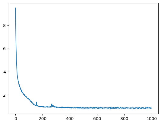
history = model.fit({"inputs": X, "targets": Y}, epochs=int(1e3), verbose=0)

plt.plot(history.history["loss"])

[<matplotlib.lines.Line2D at 0x7f63c7b639d0>]

plot(two_layer_dgp.as_prediction_model(), X, Y)

From visual inspection we immediately notice that the two-layer model performs much better.

References

[1] Silverman, B. W. (1985) “Some aspects of the spline smoothing approach to non-parametric curve fitting”. Journal of the Royal Statistical Society series B 47, 1-52.