Efficient sampling with Gaussian processes and Random Fourier Features

Gaussian processes (GPs) provide a mathematically elegant framework for learning unknown functions from data. They are robust to overfitting, allow to incorporate prior assumptions into the model and provide calibrated uncertainty estimates for their predictions. This makes them prime candidates in settings where data is scarce, noisy or very costly to obtain, and are natural tools in applications such as Bayesian optimisation (BO).

Despite their favorable properties, the use of GPs still has practical limitations. One of them is the computational complexity to draw predictive samples from the model, which quickly becomes prohibitive as the sample size grows, and creates a well-known bottleneck for GP-based Thompson sampling (GP-TS) for instance. Recent work [WBT+20] proposes to combine GP’s weight-space and function-space views to draw samples more efficiently from (approximate) posterior GPs with encouraging results in low-dimensional regimes.

In GPflux, this functionality is unlocked by grouping a kernel (e.g., gpflow.kernels.Matern52) with its feature decomposition using gpflux.sampling.KernelWithFeatureDecomposition. See the notebooks on weight space approximation and efficient posterior sampling for a thorough explanation.

import numpy as np
import tensorflow as tf
import matplotlib.pyplot as plt

import gpflow
import gpflux

from gpflow.config import default_float

from gpflux.layers.basis_functions.fourier_features import RandomFourierFeaturesCosine
from gpflux.sampling import KernelWithFeatureDecomposition
from gpflux.models.deep_gp import sample_dgp

2024-01-08 14:38:55.123460: I tensorflow/tsl/cuda/cudart_stub.cc:28] Could not find cuda drivers on your machine, GPU will not be used.
2024-01-08 14:38:55.153828: I tensorflow/tsl/cuda/cudart_stub.cc:28] Could not find cuda drivers on your machine, GPU will not be used.
2024-01-08 14:38:55.154514: I tensorflow/core/platform/cpu_feature_guard.cc:182] This TensorFlow binary is optimized to use available CPU instructions in performance-critical operations.
To enable the following instructions: AVX2 FMA, in other operations, rebuild TensorFlow with the appropriate compiler flags.

2024-01-08 14:38:55.817951: W tensorflow/compiler/tf2tensorrt/utils/py_utils.cc:38] TF-TRT Warning: Could not find TensorRT

Load Snelson dataset

d = np.load("../../tests/snelson1d.npz")
X, Y = data = d["X"], d["Y"]
num_data, input_dim = X.shape

Setting up the kernel and its feature decomposition

The KernelWithFeatureDecomposition instance represents a kernel together with its finite feature decomposition,

\[k(x, x') = \sum_{i=0}^L \lambda_i \phi_i(x) \phi_i(x'),\]

where \(\lambda_i\) and \(\phi_i(\cdot)\) are the coefficients (eigenvalues) and features (eigenfunctions), respectively, and \(L\) is the finite cutoff. See the notebook on weight space approximation for a detailed explanation of how to construct this decomposition using Random Fourier Features (RFF).

kernel = gpflow.kernels.Matern52()
Z = np.linspace(X.min(), X.max(), 10).reshape(-1, 1).astype(np.float64)

inducing_variable = gpflow.inducing_variables.InducingPoints(Z)
gpflow.utilities.set_trainable(inducing_variable, False)

num_rff = 1000
eigenfunctions = RandomFourierFeaturesCosine(kernel, num_rff, dtype=default_float())
eigenvalues = np.ones((num_rff, 1), dtype=default_float())
kernel_with_features = KernelWithFeatureDecomposition(kernel, eigenfunctions, eigenvalues)

Building and training the single-layer GP

Initialise the single-layer GP

Because KernelWithFeatureDecomposition is just a gpflow.kernels.Kernel, we can construct a GP layer with it.

layer = gpflux.layers.GPLayer(
    kernel_with_features,
    inducing_variable,
    num_data,
    whiten=True,
    num_latent_gps=1,
    mean_function=gpflow.mean_functions.Zero(),
)
likelihood_layer = gpflux.layers.LikelihoodLayer(gpflow.likelihoods.Gaussian())  # noqa: E231
dgp = gpflux.models.DeepGP([layer], likelihood_layer)
model = dgp.as_training_model()

/home/runner/work/GPflux/GPflux/gpflux/layers/gp_layer.py:198: UserWarning: Could not verify the compatibility of the `kernel`, `inducing_variable` and `mean_function`. We advise using `gpflux.helpers.construct_*` to create compatible kernels and inducing variables. As `num_latent_gps=1` has been specified explicitly, this will be used to create the `q_mu` and `q_sqrt` parameters.
  warnings.warn(
/tmp/ipykernel_2720/1062847873.py:9: DeprecationWarning: Call to deprecated class TrackableLayer. (GPflux's `TrackableLayer` was prior to TF2.5 used to collect GPflow variables in subclassed layers. As of TF 2.5, `tf.Module` supports this natively and there is no need for `TrackableLayer` anymore. It will be removed in GPflux version `1.0.0`.)
  likelihood_layer = gpflux.layers.LikelihoodLayer(gpflow.likelihoods.Gaussian())  # noqa: E231

Fit model to data

model.compile(tf.optimizers.Adam(learning_rate=0.1))

callbacks = [
    tf.keras.callbacks.ReduceLROnPlateau(
        monitor="loss",
        patience=5,
        factor=0.95,
        verbose=0,
        min_lr=1e-6,
    )
]

history = model.fit(
    {"inputs": X, "targets": Y},
    batch_size=num_data,
    epochs=100,
    callbacks=callbacks,
    verbose=0,
)

Drawing samples

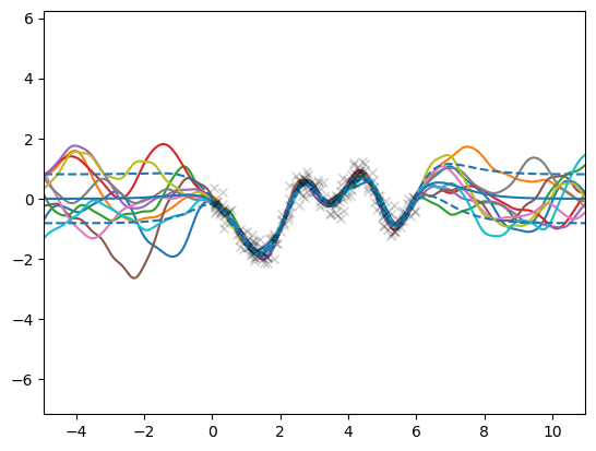
Now that the model is trained we can draw efficient and consistent samples from the posterior GP. By “consistent” we mean that the sample_dgp function returns a function object that can be evaluated multiple times at different locations, but importantly, the returned function values will come from the same GP sample. This functionality is implemented by the gpflux.sampling.efficient_sample function.

from typing import Callable

x_margin = 5
n_x = 1000
X_test = np.linspace(X.min() - x_margin, X.max() + x_margin, n_x).reshape(-1, 1)

f_mean, f_var = dgp.predict_f(X_test)
f_scale = np.sqrt(f_var)

# Plot samples
n_sim = 10
for _ in range(n_sim):
    # `sample_dgp` returns a callable - which we subsequently evaluate
    f_sample: Callable[[tf.Tensor], tf.Tensor] = sample_dgp(dgp)
    plt.plot(X_test, f_sample(X_test).numpy())

# Plot GP mean and uncertainty intervals and data
plt.plot(X_test, f_mean, "C0")
plt.plot(X_test, f_mean + f_scale, "C0--")
plt.plot(X_test, f_mean - f_scale, "C0--")
plt.plot(X, Y, "kx", alpha=0.2)
plt.xlim(X.min() - x_margin, X.max() + x_margin)
plt.ylim(Y.min() - x_margin, Y.max() + x_margin)
plt.show()