Deep Gaussian processes with Latent Variables

In this notebook, we explore the use of Deep Gaussian processes [DL13] and Latent Variables to model a dataset with heteroscedastic noise. The model can be seen as a deep GP version of [DSHD18] or as doing variational inference in models from [SDHD19]. We start by fitting a single layer GP model to show that it doesn’t result in a satisfactory fit for the noise.

This notebook is inspired by prof. Neil Lawrence’s Deep Gaussian process talk, which we highly recommend watching.

import tensorflow as tf
import gpflow
import gpflux
import numpy as np
import matplotlib.pyplot as plt
from tqdm import tqdm

import tensorflow_probability as tfp
from sklearn.neighbors import KernelDensity

Load data

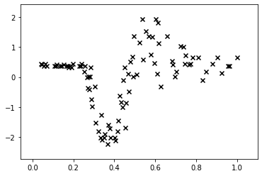
The data comes from a motorcycle accident simulation [1] and shows some interesting behaviour. In particular the heteroscedastic nature of the noise.

def motorcycle_data():
    """ Return inputs and outputs for the motorcycle dataset. We normalise the outputs. """
    import pandas as pd
    df = pd.read_csv("./data/motor.csv", index_col=0)
    X, Y = df["times"].values.reshape(-1, 1), df["accel"].values.reshape(-1, 1)
    Y = (Y - Y.mean()) / Y.std()
    X /= X.max()
    return X, Y

X, Y = motorcycle_data()
num_data, d_xim = X.shape

X_MARGIN, Y_MARGIN = 0.1, 0.5
fig, ax = plt.subplots()
ax.scatter(X, Y, marker='x', color='k');
ax.set_ylim(Y.min() - Y_MARGIN, Y.max() + Y_MARGIN);
ax.set_xlim(X.min() - X_MARGIN, X.max() + X_MARGIN);

Standard single layer Sparse Variational GP

We first show that a single layer SVGP performs quite poorly on this dataset. In the following code block we define the kernel, inducing variable, GP layer and likelihood of the shallow GP:

NUM_INDUCING = 20

kernel = gpflow.kernels.SquaredExponential()
inducing_variable = gpflow.inducing_variables.InducingPoints(
    np.linspace(X.min(), X.max(), NUM_INDUCING).reshape(-1, 1)
)
gp_layer = gpflux.layers.GPLayer(
    kernel, inducing_variable, num_data=num_data, num_latent_gps=1
)
likelihood_layer = gpflux.layers.LikelihoodLayer(gpflow.likelihoods.Gaussian(0.1))

We can now encapsulate gp_layer in a GPflux DeepGP model:

single_layer_dgp = gpflux.models.DeepGP([gp_layer], likelihood_layer)
model = single_layer_dgp.as_training_model()
model.compile(tf.optimizers.Adam(0.01))

history = model.fit({"inputs": X, "targets": Y}, epochs=int(1e3), verbose=0)
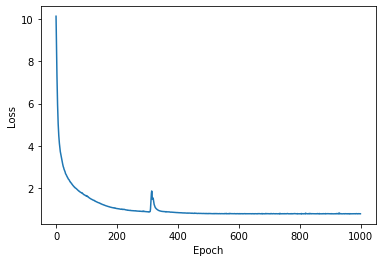
fig, ax = plt.subplots()
ax.plot(history.history["loss"])
ax.set_xlabel('Epoch')
ax.set_ylabel('Loss')

WARNING:tensorflow:From /home/vincent/anaconda3/envs/gpflow2/lib/python3.7/site-packages/tensorflow/python/ops/linalg/linear_operator_diag.py:175: calling LinearOperator.__init__ (from tensorflow.python.ops.linalg.linear_operator) with graph_parents is deprecated and will be removed in a future version.
Instructions for updating:
Do not pass `graph_parents`.  They will  no longer be used.

Text(0, 0.5, 'Loss')

fig, ax = plt.subplots()
num_data_test = 200
X_test = np.linspace(X.min() - X_MARGIN, X.max() + X_MARGIN, num_data_test).reshape(-1, 1)
model = single_layer_dgp.as_prediction_model()
out = model(X_test)

mu = out.y_mean.numpy().squeeze()
var = out.y_var.numpy().squeeze()
X_test = X_test.squeeze()

for i in [1, 2]:
    lower = mu - i * np.sqrt(var)
    upper = mu + i * np.sqrt(var)
    ax.fill_between(X_test, lower, upper, color="C1", alpha=0.3)

ax.set_ylim(Y.min() - Y_MARGIN, Y.max() + Y_MARGIN)
ax.set_xlim(X.min() - X_MARGIN, X.max() + X_MARGIN)
ax.plot(X, Y, "kx", alpha=0.5)
ax.plot(X_test, mu, "C1")
ax.set_xlabel('time')
ax.set_ylabel('acc')

Text(0, 0.5, 'acc')

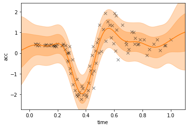
The errorbars of the single layer model are not good: we observe an overestimation of the error bars on the left and right.

Latent Variable Layer

This layer concatenates the inputs with a latent variable. See Dutordoir, Salimbeni et al. Conditional Density with Gaussian processes (2018) [DSHD18] for full details. We choose a one-dimensional input and a full parameterisation for the latent variables. This means that we do not need to train a recognition network, which is useful for fitting but can only be done in the case of small datasets, as is the case here.

w_dim = 1
prior_means = np.zeros(w_dim)
prior_std = np.ones(w_dim)
encoder = gpflux.encoders.DirectlyParameterizedNormalDiag(num_data, w_dim)
prior = tfp.distributions.MultivariateNormalDiag(prior_means, prior_std)
lv = gpflux.layers.LatentVariableLayer(prior, encoder)

First GP layer

GP Layer with two dimensional input because it acts on the inputs and the one-dimensional latent variable. We use a Squared Exponential kernel, a zero mean function, and inducing points, whose pseudo input locations are carefully chosen.

kernel = gpflow.kernels.SquaredExponential(lengthscales=[.05, .2], variance=1.)
inducing_variable = gpflow.inducing_variables.InducingPoints(
    np.concatenate(
        [
            np.linspace(X.min(), X.max(), NUM_INDUCING).reshape(-1, 1),
            np.random.randn(NUM_INDUCING, 1),
        ],
        axis=1
    )
)
gp_layer = gpflux.layers.GPLayer(
    kernel,
    inducing_variable,
    num_data=num_data,
    num_latent_gps=1,
    mean_function=gpflow.mean_functions.Zero(),
)

Second GP layer

Final layer GP with Squared Exponential kernel

kernel = gpflow.kernels.SquaredExponential()
inducing_variable = gpflow.inducing_variables.InducingPoints(
    np.random.randn(NUM_INDUCING, 1),
)
gp_layer2 = gpflux.layers.GPLayer(
    kernel,
    inducing_variable,
    num_data=num_data,
    num_latent_gps=1,
    mean_function=gpflow.mean_functions.Identity(),
)
gp_layer2.q_sqrt.assign(gp_layer.q_sqrt * 1e-5);

likelihood_layer = gpflux.layers.LikelihoodLayer(gpflow.likelihoods.Gaussian(0.01))
gpflow.set_trainable(likelihood_layer, False)
dgp = gpflux.models.DeepGP([lv, gp_layer, gp_layer2], likelihood_layer)
gpflow.utilities.print_summary(dgp, fmt="notebook")

name	class	transform	prior	trainable	shape	dtype	value
DeepGP.f_layers[0]._layers[0].means DeepGP.f_layers[0].encoder.means	Parameter	Identity		True	(94, 1)	float64	[[2.01673752e-02...
DeepGP.f_layers[0]._layers[0].stds DeepGP.f_layers[0].encoder.stds	Parameter	Softplus		True	(94, 1)	float64	[[1.e-05...
DeepGP.f_layers[1].kernel.variance	Parameter	Softplus		True	()	float64	1.0
DeepGP.f_layers[1].kernel.lengthscales	Parameter	Softplus		True	(2,)	float64	[0.05 0.2 ]
DeepGP.f_layers[1].inducing_variable.Z	Parameter	Identity		True	(20, 2)	float64	[[0.04166667, 0.66191201...
DeepGP.f_layers[1].q_mu	Parameter	Identity		True	(20, 1)	float64	[[0....
DeepGP.f_layers[1].q_sqrt	Parameter	FillTriangular		True	(1, 20, 20)	float64	[[[1., 0., 0....
DeepGP.f_layers[2].kernel.variance	Parameter	Softplus		True	()	float64	1.0
DeepGP.f_layers[2].kernel.lengthscales	Parameter	Softplus		True	()	float64	1.0
DeepGP.f_layers[2].inducing_variable.Z	Parameter	Identity		True	(20, 1)	float64	[[2.48779388...
DeepGP.f_layers[2].q_mu	Parameter	Identity		True	(20, 1)	float64	[[0....
DeepGP.f_layers[2].q_sqrt	Parameter	FillTriangular		True	(1, 20, 20)	float64	[[[1.e-05, 0.e+00, 0.e+00...
DeepGP.likelihood_layer.likelihood.variance	Parameter	Softplus + Shift		False	()	float64	0.009999999999999998

Fit

We can now fit the model. Because of the DirectlyParameterizedEncoder it is important to set the batch size to the number of datapoints and turn off shuffle. This is so that we use the associated latent variable for each datapoint. If we would use an amortized encoder network this would not be necessary.

model = dgp.as_training_model()
model.compile(tf.optimizers.Adam(0.005))
history = model.fit({"inputs": X, "targets": Y}, epochs=int(20e3), verbose=0, batch_size=num_data, shuffle=False)

gpflow.utilities.print_summary(dgp, fmt="notebook")

name	class	transform	prior	trainable	shape	dtype	value
DeepGP.f_layers[0]._metrics[0]._non_trainable_weights[0] DeepGP.f_layers[0]._metrics[0].total	ResourceVariable			False	()	float64	1.0780249257681602
DeepGP.f_layers[0]._metrics[0]._non_trainable_weights[1] DeepGP.f_layers[0]._metrics[0].count	ResourceVariable			False	()	float64	1.0
DeepGP.f_layers[0]._layers[0].means DeepGP.f_layers[0].encoder.means	Parameter	Identity		True	(94, 1)	float64	[[0.03641934...
DeepGP.f_layers[0]._layers[0].stds DeepGP.f_layers[0].encoder.stds	Parameter	Softplus		True	(94, 1)	float64	[[0.8204074...
DeepGP.f_layers[1]._metrics[0]._non_trainable_weights[0] DeepGP.f_layers[1]._metrics[0].total	ResourceVariable			False	()	float64	0.4804222860958632
DeepGP.f_layers[1]._metrics[0]._non_trainable_weights[1] DeepGP.f_layers[1]._metrics[0].count	ResourceVariable			False	()	float64	1.0
DeepGP.f_layers[1].kernel.variance	Parameter	Softplus		True	()	float64	0.8957803239319818
DeepGP.f_layers[1].kernel.lengthscales	Parameter	Softplus		True	(2,)	float64	[0.13181667 4.24491404]
DeepGP.f_layers[1].inducing_variable.Z	Parameter	Identity		True	(20, 2)	float64	[[0.10892382, -0.15883231...
DeepGP.f_layers[1].q_mu	Parameter	Identity		True	(20, 1)	float64	[[3.44379760e-02...
DeepGP.f_layers[1].q_sqrt	Parameter	FillTriangular		True	(1, 20, 20)	float64	[[[8.69748551e-02, 0.00000000e+00, 0.00000000e+00...
DeepGP.f_layers[2]._metrics[0]._non_trainable_weights[0] DeepGP.f_layers[2]._metrics[0].total	ResourceVariable			False	()	float64	0.14355680909786334
DeepGP.f_layers[2]._metrics[0]._non_trainable_weights[1] DeepGP.f_layers[2]._metrics[0].count	ResourceVariable			False	()	float64	1.0
DeepGP.f_layers[2].kernel.variance	Parameter	Softplus		True	()	float64	0.10763915659754926
DeepGP.f_layers[2].kernel.lengthscales	Parameter	Softplus		True	()	float64	0.7436233151733747
DeepGP.f_layers[2].inducing_variable.Z	Parameter	Identity		True	(20, 1)	float64	[[3.28383233e+00...
DeepGP.f_layers[2].q_mu	Parameter	Identity		True	(20, 1)	float64	[[-0.25372763...
DeepGP.f_layers[2].q_sqrt	Parameter	FillTriangular		True	(1, 20, 20)	float64	[[[9.55995241e-01, 0.00000000e+00, 0.00000000e+00...
DeepGP.likelihood_layer.likelihood.variance	Parameter	Softplus + Shift		False	()	float64	0.009999999999999998

Prediction and plotting code

Xs = np.linspace(X.min() - X_MARGIN, X.max() + X_MARGIN, num_data_test).reshape(-1, 1)

def predict_y_samples(prediction_model, Xs, num_samples=25):
    samples = []
    for i in tqdm(range(num_samples)):
        out = prediction_model(Xs)
        s = out.y_mean + out.y_var ** .5 * tf.random.normal(tf.shape(out.y_mean), dtype=out.y_mean.dtype)
        samples.append(s)
    return tf.concat(samples, axis=1)


def plot_samples(ax, N_samples=25):
    samples = predict_y_samples(dgp.as_prediction_model(), Xs, N_samples).numpy().T
    Xs_tiled = np.tile(Xs, [N_samples, 1])
    ax.scatter(Xs_tiled.flatten(), samples.flatten(), marker='.', alpha=0.2, color='C0')
    ax.set_ylim(-2.5, 2.5)
    ax.set_xlim(min(Xs), max(Xs))
    ax.scatter(X, Y, marker='.', color='C1')


def plot_latent_variables(ax):
    for l in dgp.f_layers:
        if isinstance(l, gpflux.layers.LatentVariableLayer):
            m = l.encoder.means.numpy()
            s = l.encoder.stds.numpy()
            ax.errorbar(X.flatten(), m.flatten(), yerr=s.flatten(), fmt='o')
            return

fig, (ax1, ax2) = plt.subplots(1, 2, figsize=(10, 4))
plot_samples(ax1)
plot_latent_variables(ax2)

100%|██████████| 25/25 [00:01<00:00, 24.88it/s]

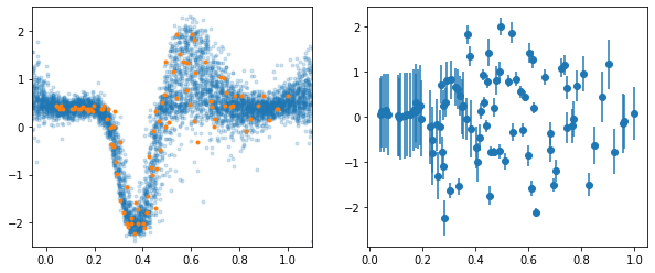
Left we show the dataset and posterior samples of \(y\). On the right we plot the mean and std. deviation of the latent variables corresponding to the datapoints.

def plot_mean_and_var(ax, samples=None, N_samples=5_000):
    if samples is None:
        samples = predict_y_samples(dgp.as_prediction_model(), Xs, N_samples).numpy().T

    m = np.mean(samples, 0).flatten()
    v = np.var(samples, 0).flatten()

    ax.plot(Xs.flatten(), m, "C1")
    for i in [1, 2]:
        lower = m - i * np.sqrt(v)
        upper = m + i * np.sqrt(v)
        ax.fill_between(Xs.flatten(), lower, upper, color="C1", alpha=0.3)
    ax.plot(X, Y, "kx", alpha=0.5)
    ax.set_ylim(Y.min() - Y_MARGIN, Y.max() + Y_MARGIN)
    ax.set_xlabel("time")
    ax.set_ylabel("acceleration")
    return samples

fig, ax = plt.subplots()
plot_mean_and_var(ax);

100%|██████████| 5000/5000 [03:24<00:00, 24.44it/s]

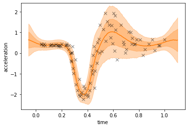
The deep GP model can handle the heteroscedastic noise in the dataset as well as the sharp-ish transition at \(0.3\).

Conclusion

In this notebook we created a two layer deep Gaussian process with a latent variable base layer to model a heteroscedastic dataset using GPflux.

[1] Silverman, B. W. (1985) “Some aspects of the spline smoothing approach to non-parametric curve fitting”. Journal of the Royal Statistical Society series B 47, 1-52.