Trust region Bayesian optimization

This notebook guides you through practical examples of trust region Bayesian optimization, illustrating algorithms like TREGO [DPRP22] and TuRBO [EPG+19] that could be beneficial for optimizing high-dimensional spaces. Trieste provides a flexible framework for implementing custom algorithms by encapsulating the behavior of rules and regions into separate abstract classes, BatchTrustRegion and UpdatableTrustRegion respectively.

Trust region optimization is a general strategy used in optimization problems where the solution space is navigated by fitting a localized model, such as a quadratic approximation, around the current point estimate and then using this model to take an optimization step. The region where this approximation is considered trustworthy is the “trust region”. Within this region, the algorithm deems the model’s predictions to be reliable enough to base decisions on. After each step, the performance of the actual function is evaluated and the trust region is adjusted accordingly – typically expanded if the model was predictive or contracted if it wasn’t.

In trust region Bayesian optimization, a probabilistic model, often a Gaussian Process, replaces simpler models like quadratics to inform the optimization. This model can be applied globally across the entire search space or adjusted to accommodate local regions.

import numpy as np
import tensorflow as tf

np.random.seed(1793)
tf.random.set_seed(1793)

Define the problem and model

We can use trust regions for Bayesian optimization in much the same way as we used EGO and EI in the introduction notebook. Since the setup is very similar to that tutorial, we’ll skip over most of the detail.

import trieste
from trieste.objectives import Branin

branin = Branin.objective
search_space = Branin.search_space

num_initial_data_points = 10
initial_query_points = search_space.sample(num_initial_data_points)
observer = trieste.objectives.utils.mk_observer(branin)
initial_data = observer(initial_query_points)

2024-11-05 17:30:50,424 INFO util.py:154 -- Missing packages: ['ipywidgets']. Run `pip install -U ipywidgets`, then restart the notebook server for rich notebook output.

As usual, we’ll use Gaussian process regression to model the function. Note that we set the likelihood variance to a small number because we are dealing with a noise-free problem.

from trieste.models.gpflow import GaussianProcessRegression, build_gpr


def build_model():
    gpflow_model = build_gpr(
        initial_data, search_space, likelihood_variance=1e-7
    )
    return GaussianProcessRegression(gpflow_model)

Trust region TREGO acquisition rule

First we demonstrate how to run Bayesian optimization with the TREGO algorithm, which alternates between regular EGO steps and local steps within one trust region (see [DPRP22]).

Create TREGO rule and run optimization loop

We can run the Bayesian optimization loop by defining a BayesianOptimizer and calling its optimize method with the trust region rule. Once the optimization loop is complete, the optimizer will return one new query point for every step in the loop; that’s 5 points in total.

The trust region rule is created by instantiating the concrete BatchTrustRegionBox class. This is a “meta” rule that manages the acquisition from multiple possible regions by applying a base-rule to each region. The default base-rule is EfficientGlobalOptimization, but a different base-rule can be provided as an argument to BatchTrustRegionBox. Here we explicitly set it to make usage clear.

The regions themselves are implemented as separate classes. The TREGO algorithm in this example requires a single region that alternates between the full search space and the trust region. This is achieved by creating one instance of the TREGOBox class, which is responsible for managing the state, initialization and update of the region.

trego_acq_rule = trieste.acquisition.rule.BatchTrustRegionBox(
    trieste.acquisition.rule.TREGOBox(search_space),
    rule=trieste.acquisition.rule.EfficientGlobalOptimization(),
)
bo = trieste.bayesian_optimizer.BayesianOptimizer(observer, search_space)

num_steps = 5
result = bo.optimize(
    num_steps, initial_data, build_model(), trego_acq_rule, track_state=True
)
dataset = result.try_get_final_dataset()

Optimization completed without errors

Visualizing TREGO results

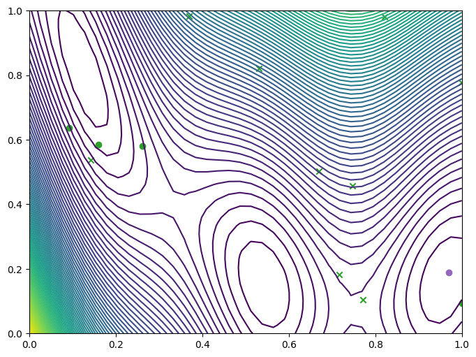
Let’s take a look at where we queried the observer, the original query points (crosses), new query points (dots) and the optimum point found (purple dot), and where they lie with respect to the contours of the Branin function.

from trieste.experimental.plotting import plot_bo_points, plot_function_2d


def plot_final_result(_dataset: trieste.data.Dataset) -> None:
    arg_min_idx = tf.squeeze(tf.argmin(_dataset.observations, axis=0))
    query_points = _dataset.query_points.numpy()
    _, ax = plot_function_2d(
        branin,
        search_space.lower,
        search_space.upper,
        grid_density=40,
        contour=True,
    )

    plot_bo_points(query_points, ax[0, 0], num_initial_data_points, arg_min_idx)


plot_final_result(dataset)

We can also visualize the progress of the optimization by plotting the acquisition space at each step. This space is either the full search space or the trust region, depending on the step, and is shown as a translucent box. The new query points per region are plotted in matching color.

Note there is only one trust region in this plot, however the rules in the following sections will show multiple trust regions.

import base64
from typing import Optional

import IPython
import matplotlib.pyplot as plt

from trieste.experimental.plotting import (
    convert_figure_to_frame,
    convert_frames_to_gif,
    plot_trust_region_history_2d,
)


def plot_history(
    result: trieste.bayesian_optimizer.OptimizationResult,
    num_query_points: Optional[int] = None,
) -> None:
    frames = []
    for step, hist in enumerate(
        result.history + [result.final_result.unwrap()]
    ):
        fig, _ = plot_trust_region_history_2d(
            branin,
            search_space.lower,
            search_space.upper,
            hist,
            num_query_points=num_query_points,
            num_init=num_initial_data_points,
        )

        if fig is not None:
            fig.suptitle(f"step number {step}")
            frames.append(convert_figure_to_frame(fig))
            plt.close(fig)

    gif_file = convert_frames_to_gif(frames)
    gif = IPython.display.HTML(
        '<img src="data:image/gif;base64,{0}"/>'.format(
            base64.b64encode(gif_file.getvalue()).decode()
        )
    )
    IPython.display.display(gif)


plot_history(result)

Batch trust region rule

Next we demonstrate how to run Bayesian optimization in a parallel batch with 5 regions.

Create the batch trust region acquisition rule

Multiple trust regions are created by providing a list of regions to the BatchTrustRegionBox rule constructor. In this example, we create 5 SingleObjectiveTrustRegionBox regions. This class encapsulates the behavior of a trust region in a single region; being responsible for maintaining its own state, initializing it, and updating it after each step. Each region contributes one query point, resulting in each acquisition step collecting 5 points overall. As the optimization process continues, the bounds of these regions are dynamically updated.

In order to perform parallel acquisition across multiple regions with BatchTrustRegionBox “meta” rule, we need to specify a batch base-rule that supports parallel optimization. For our example we use EfficientGlobalOptimization coupled with the ParallelContinuousThompsonSampling acquisition function. The batch size is controlled by the num_query_points argument.

Note: in this example the number of regions is equal to the number of batch query points in the base-rule. This results in each region contributing one query point to the overall batch. However, it is possible to generate multiple query points from each region by setting num_query_points to be a multiple Q of the number of regions. In that case, each region will contribute Q query points to the overall batch.

num_query_points = 5

init_regions = [
    trieste.acquisition.rule.SingleObjectiveTrustRegionBox(search_space)
    for _ in range(num_query_points)
]
base_rule = trieste.acquisition.rule.EfficientGlobalOptimization(  # type: ignore[var-annotated]
    builder=trieste.acquisition.ParallelContinuousThompsonSampling(),
    num_query_points=num_query_points,
)
batch_acq_rule = trieste.acquisition.rule.BatchTrustRegionBox(
    init_regions, base_rule
)

Run the optimization loop

We run the Bayesian optimization loop as before by defining a BayesianOptimizer and calling its optimize method with the trust region rule. Once the optimization loop is complete, the optimizer will return num_query_points new query points for every step in the loop. With 5 steps, that’s 25 points in total.

bo = trieste.bayesian_optimizer.BayesianOptimizer(observer, search_space)

num_steps = 5
result = bo.optimize(
    num_steps, initial_data, build_model(), batch_acq_rule, track_state=True
)
dataset = result.try_get_final_dataset()

Optimization completed without errors

Visualizing batch trust region results

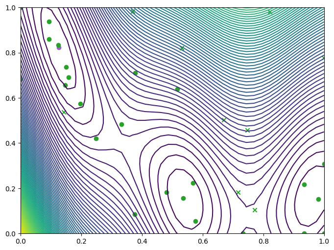
We visualize the results as before.

plot_final_result(dataset)

plot_history(result)

Trust region TuRBO acquisition rule

Finally, we show how to run Bayesian optimization with the TuRBO algorithm. This is a trust region algorithm that uses local models and datasets to approximate the objective function within their respective trust regions (see [EPG+19]).

Create TuRBO rule and run optimization loop

As before, this meta-rule requires the specification of an aquisition base-rule for performing optimization within the trust regions; for our example we use the DiscreteThompsonSampling rule.

We create 2 TuRBO trust regions and associated local models by initially copying the global model (using copy_to_local_models). The optimizer will return num_query_points new query points for each region in every step of the loop. With 5 steps and 2 regions, that’s 30 points in total.

Note: this behavior of the base-rule num_query_points argument is different from the batch-trust-region example above. In the batch-trust-region example, the total number of query points returned per step was num_query_points. In this example, the total number of query points returned per step is num_query_points * num_regions. This depends on whether the base-rule is run in parallel across all regions or in parallel only within a region. This example runs the acquisition sequentially one region at a time, wherease the batch-trust-region case performed the acquisition in parallel across all regions. Fully parallel acquisition is only supported when using EfficientGlobalOptimization base-rule without local models.

num_regions = 2
num_query_points = 3

turbo_regions = [
    trieste.acquisition.rule.TURBOBox(search_space) for _ in range(num_regions)
]
dts_rule = trieste.acquisition.rule.DiscreteThompsonSampling(
    num_search_space_samples=500, num_query_points=num_query_points
)
turbo_acq_rule = trieste.acquisition.rule.BatchTrustRegionBox(
    turbo_regions, dts_rule
)

bo = trieste.bayesian_optimizer.BayesianOptimizer(observer, search_space)

num_steps = 5
result = bo.optimize(
    num_steps,
    {trieste.observer.OBJECTIVE: initial_data},
    trieste.acquisition.utils.copy_to_local_models(build_model(), num_regions),
    turbo_acq_rule,
    track_state=True,
)
dataset = result.try_get_final_dataset()

Optimization completed without errors

Visualizing TuRBO results

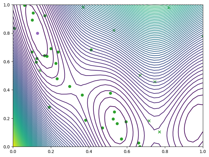
We display the results as earlier.

plot_final_result(dataset)

plot_history(result, num_regions * num_query_points)

LICENSE

Apache License 2.0