Introduction to LogEI

import numpy as np
import tensorflow as tf
import trieste

np.random.seed(1794)
tf.random.set_seed(1794)

2025-09-24 09:20:55,833 INFO util.py:154 -- Missing packages: ['ipywidgets']. Run `pip install -U ipywidgets`, then restart the notebook server for rich notebook output.

What is LogEI?

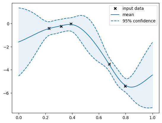
LogEI ([ADE+23]) is the improved version of expected improvement (EI), which shares the same optima as original EI while is substantially easier to optimize numerically. To see the difference, let’s use the following simple setting.

import matplotlib.pyplot as plt
import gpflow
from trieste.models.gpflow import GaussianProcessRegression, build_gpr


## Defining a problem
def forrester_true(x):
    return (6.0 * x - 2) ** 2 * tf.sin(12.0 * x - 4)


def forrester_sim(x):
    y = forrester_true(x)
    noise = tf.random.normal(y.shape, 0.0, 0.25, dtype=y.dtype)
    return y + noise


search_space = trieste.space.Box([0.0], [1.0])
f_observer = trieste.objectives.utils.mk_observer(forrester_sim)

## Build gpflow model

n = 5
X = np.random.default_rng(12345).random((n, 1))
data = f_observer(X)
gpflow_m = build_gpr(data, search_space)
optimiser = gpflow.optimizers.Scipy()
optimiser.minimize(gpflow_m.training_loss, gpflow_m.trainable_variables)
m = GaussianProcessRegression(gpflow_m)

## Plot data and model prediction
Xplot = np.linspace(0, 1.0, 100)[:, None]
y_mean, y_var = m.predict_y(Xplot)
y_lower = y_mean - 1.96 * np.sqrt(y_var)
y_upper = y_mean + 1.96 * np.sqrt(y_var)

plt.plot(data.query_points, data.observations, "kx", mew=2, label="input data")
plt.plot(Xplot, y_mean, "-", color="C0", label="mean")
plt.plot(Xplot, y_lower, "--", color="C0", label="95% confidence")
plt.plot(Xplot, y_upper, "--", color="C0")
plt.fill_between(
    Xplot[:, 0], y_lower[:, 0], y_upper[:, 0], color="C0", alpha=0.1
)
plt.legend()

<matplotlib.legend.Legend at 0x7fded060fe50>

We can compute the original EI and logEI on this GP model. Note that we use different axis for each aquisition function for the ease of comparison.

from trieste.acquisition.function import (
    ExpectedImprovement,
    LogExpectedImprovement,
)

acq_EI_func = ExpectedImprovement().prepare_acquisition_function(m, data)
acq_logEI_func = LogExpectedImprovement().prepare_acquisition_function(m, data)


X_grid = np.linspace(0.0, 1.0, 100)

log_EI_val = acq_logEI_func(X_grid[:, None, None])
EI_val = acq_EI_func(X_grid[:, None, None])


def plot_EI_and_logEI(X_grid, log_EI_val, EI_val):
    fig, ax1 = plt.subplots()
    color = "tab:red"
    ax1.set_xlabel("x")
    ax1.set_ylabel("logEI", color=color)
    ax1.plot(X_grid, log_EI_val[:, 0], color=color, label="logEI")
    ax1.tick_params(axis="y", labelcolor=color)

    ax2 = ax1.twinx()

    color = "tab:blue"
    ax2.set_ylabel("EI", color=color)
    ax2.plot(X_grid, EI_val[:, 0], color=color, label="EI")
    ax2.tick_params(axis="y", labelcolor=color)

    lines_labels = [ax.get_legend_handles_labels() for ax in fig.axes]
    lines, labels = [sum(lol, []) for lol in zip(*lines_labels)]
    fig.legend(lines, labels, loc="lower right", bbox_to_anchor=(0.87, 0.15))
    fig.tight_layout()


plot_EI_and_logEI(X_grid, log_EI_val, EI_val)

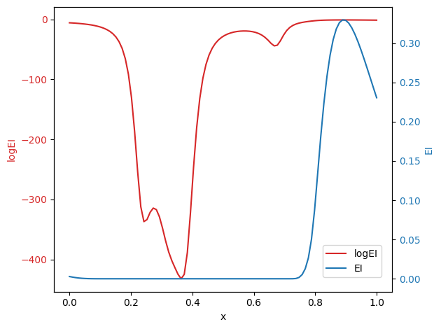
We can see that EI has the large flat region with the zero value, which makes it challenging to optimize by gradient-based algorithms. This issue is mitigated by the logEI, which has non-zero gradient for most of regions. To see the performance, we replicate the Sum-of-Squares (SoS) function experiment presented in the logEI paper.

from trieste.experimental.plotting import plot_regret
from trieste.acquisition.rule import EfficientGlobalOptimization


## Defining a SoS problem
def SoS(x):
    return tf.reduce_sum((x - 0.5) ** 2, keepdims=True, axis=1)


def benchmark_SoS(
    search_space, observer, acq_rule_builder, initial_data, n_step, ax
):

    gpflow_model = trieste.models.gpflow.build_gpr(
        initial_data, search_space, likelihood_variance=1e-7
    )
    model = trieste.models.gpflow.GaussianProcessRegression(
        gpflow_model, num_kernel_samples=100
    )

    bo = trieste.bayesian_optimizer.BayesianOptimizer(observer, search_space)
    acq_rule = EfficientGlobalOptimization(builder=acq_rule_builder)
    results = bo.optimize(
        n_step, initial_data, model, acquisition_rule=acq_rule
    )

    # plotting
    dataset = results.try_get_final_dataset()
    query_points = dataset.query_points.numpy()
    observations = dataset.observations.numpy()

    _, min_obs, arg_min_idx = results.try_get_optimal_point()
    suboptimality = observations  # the true optimal score is zero
    plot_regret(
        suboptimality, ax, num_init=num_initial_points, idx_best=arg_min_idx
    )
    ax.set_ylim([1.0e-4, 2.0])
    ax.set_yscale("log")

    return min_obs[0]


num_initial_points = 10
n_step = 50
ndim = 10
search_space = trieste.space.Box([0.0] * ndim, [1.0] * ndim)
observer = trieste.objectives.utils.mk_observer(SoS)

initial_query_points = search_space.sample_sobol(num_initial_points)
initial_data = observer(initial_query_points)

fig, ax = plt.subplots(1, 2)
EI_min_obs = benchmark_SoS(
    search_space,
    observer,
    trieste.acquisition.function.ExpectedImprovement(),
    initial_data,
    n_step,
    ax[0],
)
ax[0].set_title(f"Regret for EI \n (min = {EI_min_obs:.2e})")


log_EI_min_obs = benchmark_SoS(
    search_space,
    observer,
    trieste.acquisition.function.LogExpectedImprovement(),
    initial_data,
    n_step,
    ax[1],
)
ax[1].set_title(f"Regret for LogEI \n (min = {log_EI_min_obs:.2e})")

fig.tight_layout()

Optimization completed without errors
Optimization completed without errors

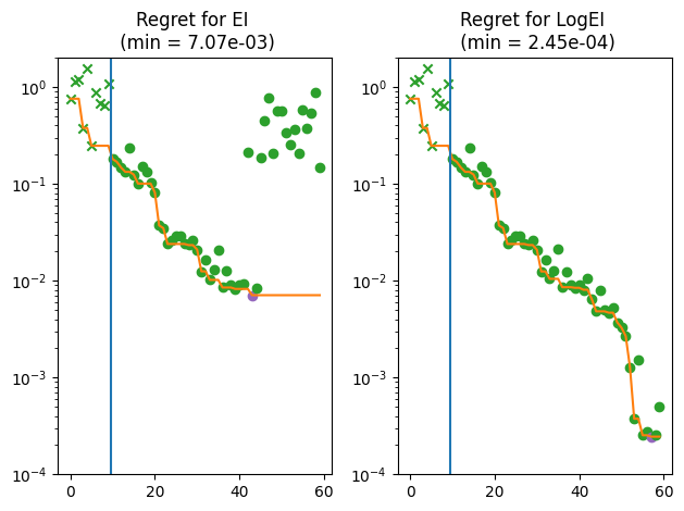
From the figure, we can tell that EI becomes unable to find better points after several observations even on this trivial problem, while logEI makes steady improvement throughout the process. A similar log-trick can be also applied to other EI family of acquisition functions including LogAugmentedExpectedImprovement.

LICENSE

Apache License 2.0