Multifidelity Modelling with Autoregressive Model

This tutorial demonstrates the usage of the MultifidelityAutoregressive model for fitting multifidelity data. This is an implementation of the AR1 model initially described in [KOHagan00].

import tensorflow as tf
import numpy as np
import matplotlib.pyplot as plt

np.random.seed(1793)
tf.random.set_seed(1793)

Describe the problem

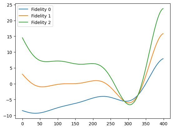
In this tutorial we will consider the scenario where we have a simulator that can be run at three fidelities, with the ability to get cheap but coarse results at the lowest fidelity, more expensive but more refined results at a middle fidelity and very accurate but very expensive results at the highest fidelity.

We define the true functions for the fidelities as:

\[f_{i} : [0, 1] \rightarrow \mathbb{R}\]

\[f_0(x) = \frac{\sin(12x -4)(6x - 2)^2 + 10(x-1)}{2}, \quad x \in [0,1]\]

\[f_i(x) = f_{i-1}(x) + i(f_{i-1}(x) - 20(x - 1)), \quad x \in [0,1] , \quad i \in \mathbb{N}\]

Note that noise is optionally added to any observations in all but the lowest fidelity. There are a few modelling assumptions: 1. The lowest fidelity is noise-free 2. The data is cascading, e.g any point that has an observation at a high fidelity also has one at the lower fidelities.

# Define the multifidelity simulator
def simulator(x_input, fidelity, add_noise=False):

    f = 0.5 * ((6.0 * x_input - 2.0) ** 2) * tf.math.sin(
        12.0 * x_input - 4.0
    ) + 10.0 * (x_input - 1.0)
    f = f + fidelity * (f - 20.0 * (x_input - 1.0))
    if add_noise:
        noise = tf.random.normal(f.shape, stddev=1e-1, dtype=f.dtype)
    else:
        noise = 0
    f = tf.where(fidelity > 0, f + noise, f)
    return f


# Plot the fidelities
x = np.linspace(0, 1, 400)

y0 = simulator(x, 0)
y1 = simulator(x, 1)
y2 = simulator(x, 2)

plt.plot(y0, label="Fidelity 0")
plt.plot(y1, label="Fidelity 1")
plt.plot(y2, label="Fidelity 2")
plt.legend()
plt.show()

Trieste handles fidelities by adding an extra column to the data containing the fidelity information of the query point. The function check_and_extract_fidelity_query_points will check that the fidelity column is valid, and if so, will separate the query points and the fidelity information.

from trieste.data import Dataset, check_and_extract_fidelity_query_points

# Create an observer class to deal with multifidelity input query points
class Observer:
    def __init__(self):

        self.simulator = simulator

    def __call__(self, x, add_noise=True):

        # Extract raw input and fidelity columns
        x_input, x_fidelity = check_and_extract_fidelity_query_points(x)

        # note: this assumes that my_simulator broadcasts, i.e. accept matrix inputs.
        # If not you need to replace this by a for loop over all rows of "input"
        observations = self.simulator(x_input, x_fidelity, add_noise)
        return Dataset(query_points=x, observations=observations)


# Instantiate the observer
observer = Observer()

/opt/hostedtoolcache/Python/3.7.15/x64/lib/python3.7/site-packages/gpflow/experimental/utils.py:43: UserWarning: You're calling gpflow.experimental.check_shapes.decorator.check_shapes which is considered *experimental*. Expect: breaking changes, poor documentation, and bugs.
  f"You're calling {name} which is considered *experimental*."
/opt/hostedtoolcache/Python/3.7.15/x64/lib/python3.7/site-packages/gpflow/experimental/utils.py:43: UserWarning: You're calling gpflow.experimental.check_shapes.inheritance.inherit_check_shapes which is considered *experimental*. Expect: breaking changes, poor documentation, and bugs.
  f"You're calling {name} which is considered *experimental*."

Now we can define the other parameters of our problem, such as the input dimension, search space and number of fidelities.

from trieste.space import Box

input_dim = 1
n_fidelities = 3

lb = np.zeros(input_dim)
ub = np.ones(input_dim)

input_search_space = Box(lb, ub)

Create initial dataset

from trieste.data import add_fidelity_column

# Define sample sizes of low, mid and high fidelities
sample_sizes = [18, 12, 6]

xs = [tf.linspace(0, 1, sample_sizes[0])[:, None]]

# Take a subsample of each lower fidelity to sample at the next fidelity up
for fidelity in range(1, n_fidelities):
    samples = tf.Variable(
        np.random.choice(
            xs[fidelity - 1][:, 0], size=sample_sizes[fidelity], replace=False
        )
    )[:, None]
    xs.append(samples)
# Add fidelity columns to training data
initial_samples_list = [add_fidelity_column(x, i) for i, x in enumerate(xs)]

initial_sample = tf.concat(initial_samples_list, 0)
initial_data = observer(initial_sample, add_noise=True)

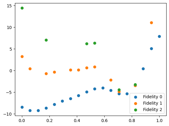
We can plot the initial data. We separate the dataset into individual fidelities using the split_dataset_by_fidelity function.

from trieste.data import split_dataset_by_fidelity

data = split_dataset_by_fidelity(initial_data, num_fidelities=n_fidelities)

plt.scatter(data[0].query_points, data[0].observations, label="Fidelity 0")
plt.scatter(data[1].query_points, data[1].observations, label="Fidelity 1")
plt.scatter(data[2].query_points, data[2].observations, label="Fidelity 2")
plt.legend()
plt.show()

Now we can fit the MultifidelityAutoregressive model to this data. We use the build_multifidelity_autoregressive_models to create the sub-models required by the multifidelity model.

from trieste.models.gpflow import (
    MultifidelityAutoregressive,
    build_multifidelity_autoregressive_models,
)

# Initialise model
multifidelity_model = MultifidelityAutoregressive(
    build_multifidelity_autoregressive_models(
        initial_data, n_fidelities, input_search_space
    )
)

# Update and optimize model
multifidelity_model.update(initial_data)
multifidelity_model.optimize(initial_data)

/opt/hostedtoolcache/Python/3.7.15/x64/lib/python3.7/site-packages/gpflow/experimental/utils.py:43: UserWarning: You're calling gpflow.experimental.check_shapes.checker.ShapeChecker.__init__ which is considered *experimental*. Expect: breaking changes, poor documentation, and bugs.
  f"You're calling {name} which is considered *experimental*."

Plot Results

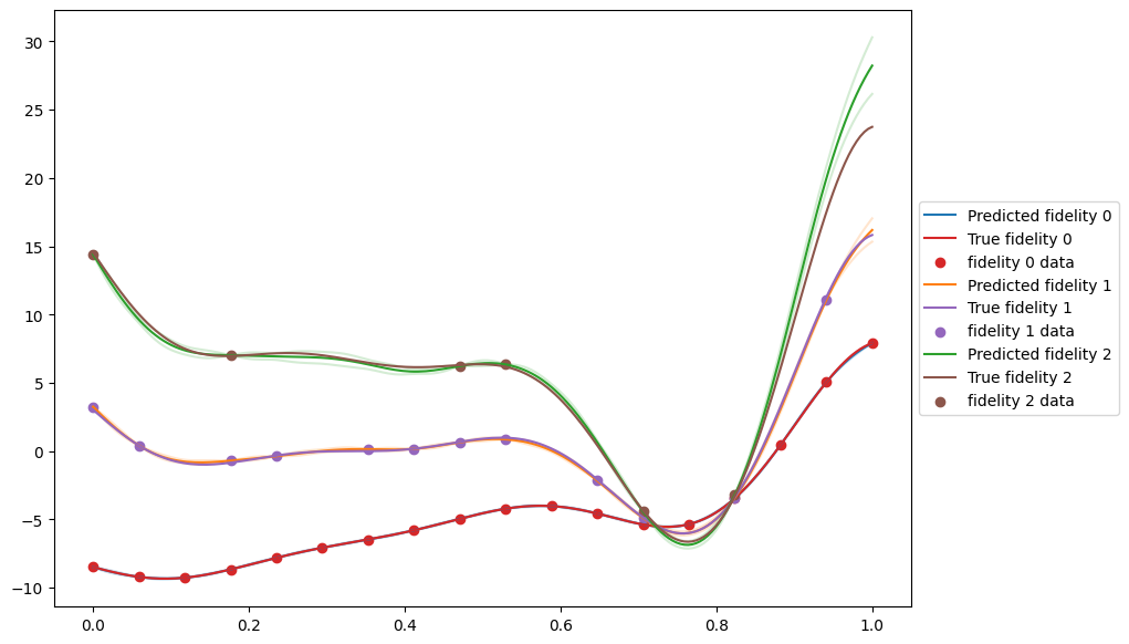
Now we can plot the results to have a look at the fit. The MultifidelityAutoregressive.predict method requires data with a fidelity column that specifies the fidelity for each data point to be predicted at. We use the add_fidelity_column function to add this.

X = tf.linspace(0, 1, 200)[:, None]
X_list = [add_fidelity_column(X, i) for i in range(n_fidelities)]
predictions = [multifidelity_model.predict(x) for x in X_list]

fig, ax = plt.subplots(1, 1, figsize=(10, 7))

pred_colors = ["tab:blue", "tab:orange", "tab:green"]
gt_colors = ["tab:red", "tab:purple", "tab:brown"]

for fidelity, prediction in enumerate(predictions):
    mean, var = prediction
    ax.plot(
        X,
        mean,
        label=f"Predicted fidelity {fidelity}",
        color=pred_colors[fidelity],
    )
    ax.plot(
        X,
        mean + 1.96 * tf.math.sqrt(var),
        alpha=0.2,
        color=pred_colors[fidelity],
    )
    ax.plot(
        X,
        mean - 1.96 * tf.math.sqrt(var),
        alpha=0.2,
        color=pred_colors[fidelity],
    )
    ax.plot(
        X,
        observer(X_list[fidelity], add_noise=False).observations,
        label=f"True fidelity {fidelity}",
        color=gt_colors[fidelity],
    )
    ax.scatter(
        data[fidelity].query_points,
        data[fidelity].observations,
        label=f"fidelity {fidelity} data",
        color=gt_colors[fidelity],
    )
ax.legend(loc="center left", bbox_to_anchor=(1, 0.5))
plt.show()

Comparison with naive model fit on high fidelity

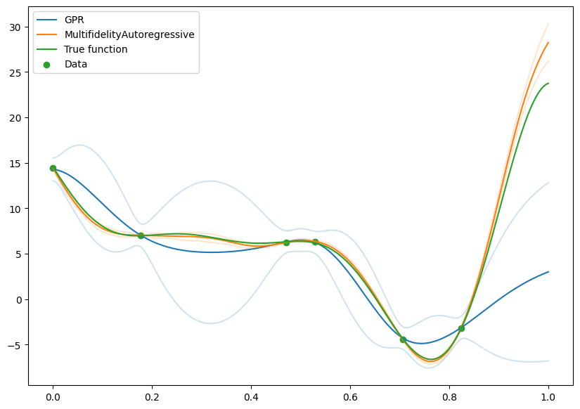
We can compare with a model that was fit just on the high fidelity data, and see the gains from using the low fidelity data.

from trieste.models.gpflow import GaussianProcessRegression, build_gpr
from trieste.data import add_fidelity_column

# Get high fidleity data
hf_data = data[2]

# Fit simple gpr model to high fidelity data
gpr_model = GaussianProcessRegression(build_gpr(hf_data, input_search_space))

gpr_model.update(hf_data)
gpr_model.optimize(hf_data)

X = tf.linspace(0, 1, 200)[:, None]
# Turn X into high fidelity query points for the multifidelity model
X_for_multifid = add_fidelity_column(X, 2)

gpr_predictions = gpr_model.predict(X)
multifidelity_predictions = multifidelity_model.predict(X_for_multifid)

fig, ax = plt.subplots(1, 1, figsize=(10, 7))

"tab:blue", "tab:orange", "tab:green"

# Plot gpr results
mean, var = gpr_predictions
ax.plot(X, mean, label=f"GPR", color="tab:blue")
ax.plot(X, mean + 1.96 * tf.math.sqrt(var), alpha=0.2, color="tab:blue")
ax.plot(X, mean - 1.96 * tf.math.sqrt(var), alpha=0.2, color="tab:blue")

# Plot gpr results
mean, var = multifidelity_predictions
ax.plot(X, mean, label=f"MultifidelityAutoregressive", color="tab:orange")
ax.plot(X, mean + 1.96 * tf.math.sqrt(var), alpha=0.2, color="tab:orange")
ax.plot(X, mean - 1.96 * tf.math.sqrt(var), alpha=0.2, color="tab:orange")


# Plot true function
ax.plot(
    X,
    observer(X_for_multifid, add_noise=False).observations,
    label=f"True function",
    color="tab:green",
)

# Scatter the data
ax.scatter(
    hf_data.query_points, hf_data.observations, label=f"Data", color="tab:green"
)
plt.legend()
plt.show()

It’s clear that there is a large benefit to being able to make use of the low fidelity data, and this is particularly noticable in the greatly reduced confidence intervals.