Mixed search spaces

This notebook demonstrates optimization of mixed search spaces in Trieste.

The example function is defined over 2D input space that is a combination of a discrete and a continuous search space. The problem is a modification of the Branin function where one of the input dimensions is discretized.

import numpy as np
import tensorflow as tf

np.random.seed(1793)
tf.random.set_seed(1793)

The problem

The Branin function is a common optimization benchmark that has three global minima. It is normally defined over a 2D continuous search space.

We first show the Branin function over its original continuous search space.

from trieste.experimental.plotting import plot_function_plotly
from trieste.objectives import ScaledBranin

scaled_branin = ScaledBranin.objective

fig = plot_function_plotly(
    scaled_branin,
    ScaledBranin.search_space.lower,
    ScaledBranin.search_space.upper,
)
fig.show()

In order to convert the Branin function from a continuous to a mixed search space problem, we modify it by discretizing its first input dimension.

The discrete dimension is defined by a set of 10 points that are equally spaced, ensuring that the three minimizers are included in this set. The continuous dimension is defined by the interval [0, 1].

We observe that the first and third minimizers are equidistant from the middle minimizer, so we choose the discretization points to be equally spaced around the middle minimizer.

The TaggedProductSearchSpace class is a convenient way to define a search space that is a combination of multiple search spaces, each with an optional tag. We create our mixed search space by instantiating this class with a list containing the discrete and continuous spaces, without any explicit tags (hence using default tags). This can be easily extended to more than two search spaces by adding more elements to the list.

from trieste.space import Box, DiscreteSearchSpace, TaggedProductSearchSpace

minimizers0 = ScaledBranin.minimizers[:, 0]
step = (minimizers0[1] - minimizers0[0]) / 4
points = np.concatenate(
    [
        # Equally spaced points to the left of the middle minimizer. Skip the last point as it is
        # the same as the first point in the next array.
        np.flip(np.arange(minimizers0[1], 0.0, -step))[:-1],
        # Equally spaced points to the right of the middle minimizer.
        np.arange(minimizers0[1], 1.0, step),
    ]
)
discrete_space = DiscreteSearchSpace(points[:, None])
continuous_space = Box([0.0], [1.0])
mixed_search_space = TaggedProductSearchSpace(
    [discrete_space, continuous_space]
)

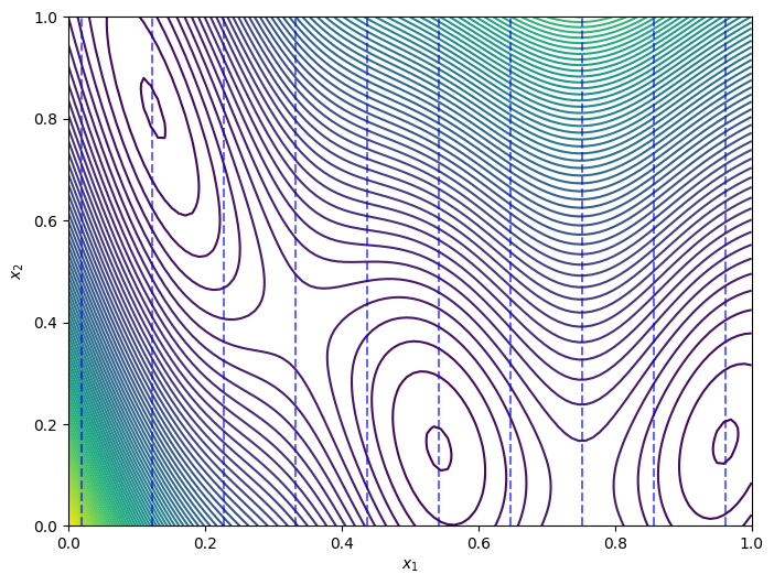
Next we demonstrate the Branin function over the mixed search space, by plotting the original function contours and highlighting the discretization points. The discrete dimension is along the x-axis and the continuous dimension is on the y-axis, with the vertical dashed lines indicating the discretization points.

from trieste.experimental.plotting import plot_function_2d

# Plot over the predefined search space.
fig, ax = plot_function_2d(
    scaled_branin,
    ScaledBranin.search_space.lower,
    ScaledBranin.search_space.upper,
    contour=True,
)

ax[0, 0].set_xlabel(r"$x_1$")
ax[0, 0].set_ylabel(r"$x_2$")

# Draw vertical lines at the discrete points.
for point in points:
    ax[0, 0].vlines(
        point,
        mixed_search_space.lower[1],
        mixed_search_space.upper[1],
        colors="b",
        linestyles="dashed",
        alpha=0.6,
    )

/opt/hostedtoolcache/Python/3.10.13/x64/lib/python3.10/site-packages/matplotlib/_mathtext.py:1880: UserWarning:

warn_name_set_on_empty_Forward: setting results name 'sym' on Forward expression that has no contained expression

/opt/hostedtoolcache/Python/3.10.13/x64/lib/python3.10/site-packages/matplotlib/_mathtext.py:1885: UserWarning:

warn_ungrouped_named_tokens_in_collection: setting results name 'name' on ZeroOrMore expression collides with 'name' on contained expression

Sample the observer over the search space

We begin our optimization by first collecting five function evaluations from random locations in the mixed search space. Samples from the discrete dimension are drawn uniformly at random with replacement, and samples from the continuous dimension are drawn from a uniform distribution. Observe that the sample method deals with the mixed search space automatically.

from trieste.objectives import mk_observer

observer = mk_observer(scaled_branin)

num_initial_points = 5
initial_query_points = mixed_search_space.sample(num_initial_points)
initial_data = observer(initial_query_points)

Model the objective function

We now build a Gaussian process model of the objective function using the initial data, similar to the introduction notebook.

Since all of the data in this example is quantitative, the model does not differentiate between the discrete and continuous dimensions of the search space. The Gaussian process regression model treats all dimensions as continuous variables, allowing for a seamless integration of both types of dimensions in the optimization process.

from trieste.models.gpflow import GaussianProcessRegression, build_gpr

gpflow_model = build_gpr(
    initial_data, mixed_search_space, likelihood_variance=1e-7
)
model = GaussianProcessRegression(gpflow_model)

Run the optimization loop

The Bayesian optimization loop is run for 15 steps over the mixed search space. For each step, the optimizer fixes the discrete dimension to the best points found from a random initial search, and then optimizes the continuous dimension using a gradient-based method. This dispatch of discrete and continuous optimization is handled by the optimizer automatically.

from trieste.bayesian_optimizer import BayesianOptimizer

bo = BayesianOptimizer(observer, mixed_search_space)

num_steps = 15
result = bo.optimize(num_steps, initial_data, model)
dataset = result.try_get_final_dataset()

Optimization completed without errors

Explore the results

We can now get the best point found by the optimizer. Note that this isn’t necessarily the last evaluated point.

query_point, observation, arg_min_idx = result.try_get_optimal_point()

print(f"query point: {query_point}")
print(f"observation: {observation}")

query point: [0.54277284 0.16439408]
observation: [-1.04669231]

The plot below highlights how the optimizer explored the mixed search space over the course of the optimization loop. The green ‘x’ markers indicate the initial points, the green circles mark the points evaluated during the optimization loop, and the purple circle indicates the optimal point found by the optimizer.

from trieste.experimental.plotting import plot_bo_points

query_points = dataset.query_points.numpy()
observations = dataset.observations.numpy()

_, ax = plot_function_2d(
    scaled_branin,
    ScaledBranin.search_space.lower,
    ScaledBranin.search_space.upper,
    contour=True,
)
plot_bo_points(query_points, ax[0, 0], num_initial_points, arg_min_idx)
ax[0, 0].set_xlabel(r"$x_1$")
ax[0, 0].set_ylabel(r"$x_2$")

for point in points:
    ax[0, 0].vlines(
        point,
        mixed_search_space.lower[1],
        mixed_search_space.upper[1],
        colors="b",
        linestyles="dashed",
        alpha=0.6,
    )

LICENSE

Apache License 2.0